Proceedings of the UGV Technology Conference at the 2003 SPIE AeroSense Symposium, Orlando, FL, April 21-25, 2003
Reduction of Odometry Errors in Over-constrained Mobile Robots
1
by
Lauro Ojeda and Johann Borenstein University of Michigan 1101 Beal Ave. Ann Arbor, MI 48109
[email protected] and
[email protected]
ABSTRACT This paper presents an analysis of odometry errors in over-constrained mobile robots, that is, vehicles that have more independent motors than degrees of freedom. Based on our analysis we developed and examined three novel error-reducing methods. One method, called “Fewest Pulses” method, makes use of the observation that most terrain irregularities, as well as wheel slip, result in an erroneous over-count of encoder pulses. A second method, called “Cross-coupled Control,” optimizes the motor control algorithm of the robot to reduce synchronization errors that would otherwise result in wheel slip with conventional controllers. The third method is based on so-called Expert Rules. With this method readings from redundant encoders are compared and utilized in different ways, according to predefined rules. In the work described here we implemented our three error reducing methods on a modified Pioneer AT skid-steer platform and compared their odometric accuracy. The results in this paper point to clear advantages of the Expert Rulebased method over the other tested methods. Keywords: Mobile Robot, Odometry, Error correction, Cross-coupled Control, Expert Rules, Pioneer AT, Overconstrained, Encoders
1
INTRODUCTION AND STATEMENT OF PROBLEM
Land vehicles with more than three kinematically independent motors are defined2 as over-constrained because there are only three degrees of freedom of motion for land vehicles. In earlier work we analyzed and discussed the ill-effects of over-constrained kinematic designs on odometric accuracy and we provided the solution of the so-called “compliant linkage” to eliminate the problem for certain platform designs with four drive motors [Borenstein, 1995]. Many mobile robots have even more independent motors for driving and steering. For example, the Mars Rovers Rocky-8 and Fido, which were designed and built by the Jet Propulsion Labs [JPL 2002], have six independently controlled drive motors and six independently controlled steering motors for their six wheels. Other examples of mobile robots with over-constrained drive systems are the six-wheeled SHRIMP made by Bluebotics [2002], the Nomad arctic traverse robot developed at Carnegie Mellon University [Shamah et al., 1998], and wheeled snake-type robots like the ones developed by Hirose et al. [1991]. For all of these vehicles the designers accept the reduction of odometric accuracy in their over-constrained systems as a tradeoff for increased mobility. This paper analyses some aspects of odometry errors in these over-constrained mobile robots and proposed improvements that can be applied without the need for mechanical redesign. To do so we turned our attention to the 4-wheeldrive/skid-steer (4WDSS) mobile robots of the Pioneer-series [Activemedia 2002] and the ATRV-series [iRobot 2002]. Interestingly the manufacturers of these robots chose to drive the wheels on each side of these platforms by two kine-
1 2
This paper is a shortened version of a manuscript submitted for publication to the Journal of Autonomous Robots in 12/2002.
This is a simplified definition that is suitable for the purpose and scope of this paper. An in-depth treatment of vehicle kinematics, degrees of freedom, and constrains is presented in [Muir and Neuman, 1987].
matically linked electric motors, thereby providing a total of four drive motors in each vehicle. However, since the two motors on each side are mechanically linked to each other by belts or chains, the two motors on each side act as one. In order to create an over-constrained platform for our experiments we simply removed the drive belts from the motor pairs on each side of an off-theshelf Pioneer AT platform. We also equipped the two originally encoderless motors with incremental optical encoders. The result was the platform shown in Figure 1. Using this modified configuration of the Pioneer ATbased platform we investigated several methods for reducing odometry errors in over-constrained mobile robots, as explained in Section 2. Experimental results are provided in Section 3 and Conclusions are presented in Section 4.
2
METHODS FOR REDUCING ODOMETRY ERRORS
Figure 1: UM’s modified Pioneer AT with redundant encoders.
In this section we present three candidate methods for reducing odometry errors. We called them: (1) The “Fewest Pulses” method, (2) the “Cross-coupled Control” method, and (3) the “Expert Rules” method. 2.1 The Fewest Pulses method Since only two encoders are needed to compute basic odometry, four encoders, as used in our modified Pioneer AT, are redundant. One somewhat obvious approach to arbitration among redundant encoders is to apply a simple rule: “Use only the data from the encoder-pair3 that provided the least number of pulses during the last sampling interval.” The rationale behind this approach is that for most error-causing conditions encoders “over-count.” That is, they provide more pulses than what corresponds to the actual linear distance traveled, when they encounter wheel slip or bumps or cracks on the ground. However, in our work we soon discovered that there is a technical caveat with this approach. The caveat is related to the rounding error inherent in measuring wheel rotation with incremental encoders. To explain this effect, consider a conventional differential-drive mobile robot with a total of just two wheel encoders, where the same two encoders are sampled for odometry during each sampling interval. Since encoder pulses are discrete events, sampling might produce a number like, say, 35 pulses for a given sampling interval, even though the actual rotation of the wheel might have corresponded to, say, 35.6 pulses. The truncated .6 pulses are no problem, because they go into the next encoder sample, which would read 36 pulses, even though the wheel rotation during that next sampling interval might still have corresponded to only 35.6 pulses (at constant speed, etc.). However, when the Fewest Pulses Method is applied in our redundant encoder system, then it is not the same encoder that gets sampled every time, and which would therefore carry over a truncated fraction into the next sampling interval. Rather, since we always select the encoder with the smallest number of pulses in a sampling interval, we would always select the encoder that reads 35 pulses, while the other encoder might read 36 pulses (to stick with the above example). Furthermore, since this decision causes an unrecovered truncation error every time we sample, the overall error can be rather large. It is possible to correct for the truncation error as follows. Obviously, the truncation error is always an amount between 0.0 and 1.0; on average 0.5. Furthermore, the truncation error always results in an underestimation of distance traveled. We can thus reduce the effect of the truncation error by adding a correction factor of c = 0.5 to the reading of the encoder with the fewest pulses, whenever readings are switched from one encoder to the other on that side and a difference exist between both encoders. Under most conditions this approach is quite effective. However, as we mentioned earlier, the Fewest Pulses Method doesn’t apply to all conditions, as discussed in the next section. 3 An “encoder-pair” in our redundant system is comprised of one encoder from the right side and one from the left side. An encoder pair could thus comprise, for example, the left front encoder and the rear right encoder.
2
2.2 The Cross-coupled Control method At low speeds (e.g., slower than 200 mm/sec) and while driving over a low traction surface like sand, we observed that there is actually rather significant wheel skid4. Skidding is different from slipping in that skidding wheels always produce fewer encoder pulses than tracking wheels, while slipping wheels produce more encoder pulses than tracking wheels. Our analysis revealed that there are two causes for the excessive wheel skid in over-constrained robots: 1. In conventional motion control for differential-drive vehicles the software prescribes separate reference velocities to the left and right wheels. Under normal conditions there are short transient times, during which the motors try to get up to the commanded speed; and then, if the control loop is properly designed, the wheels settle at their commanded speed. However, external disturbances and slippage will interfere with the commanded speeds and result in additional transient times, during which the wheels don’t follow the commanded speeds exactly. This situation is exacerbated when driving at very slow speeds, because then internal friction in gears and bearings causes significant disturbances all the time and oftentimes halts a wheel altogether. 2. In differential-drive mobile robots, such as the venerable LabMate platform, momentary deviations from commanded speeds only reduce the accuracy, at which the robot tracks a given path. This is not a big problem in most applications. However, in a skid-steer platform like the Pioneer AT the problem is much more severe. This is because the four-wheel drive Pioneer AT is mathematically severely over-constrained, that is, it has four controlled motors but only one independent degree of freedom: forward/backward motion. As a result, all wheels have to run at the exact same speed to avoid slippage. Yet, even when commanded to move straight forward, any momentary mismatch between wheel velocities will force the wheels to skid or slip unpredictably. One way to reduce the occurrence of slippage in over-constrained vehicles is the use of the so-called “Cross-coupled Control” (CCC) method. This method was originally developed by Borenstein and Koren [1985; 1987] and later refined by Feng, Koren, and Borenstein [1993]. The CCC method continuously compares the actual encoder pulses from the left and right wheel of a robot and issues corrective commands to the motors to slow down the motor that is faster and speed up the motor that is slower than the other. The overall effect of this method is that the velocities of the left and right wheels of a robot are matched more tightly even in the presence of internal and external disturbances. Figure 2 shows a block diagram with the implementation of cross-coupled control between the left-front and left-rear motor. Conventional motor control loop, front motor Front wheel speed command
+
+
DAC
Amplifier
Motor
Front wheel position
-
Cross-coupled controller
Encoder
+ PI Controller
Encoder
+
+
+
DAC
Amplifier
Motor
Rear wheel speed command
Rear wheel position
Conventional motor control loop, rear motor
Figure 2: Block diagram of Cross-coupled Control (CCC), here shown for the two left-hand wheels. 4
Because of ambiguity in the way the terms slip and skid are used in the scientific literature, we define these terms in the context of this paper as follows: “Slip” or “slipping” is the loss of traction that results when the motor applies too much power to the wheel, e.g., over-acceleration. “Skid” or “skidding” is the loss of traction that results when the vehicle is in motion but a wheel is blocked or partially blocked from rolling by excessive friction in the drive train or the effect of motor braking. We refer to slip and skid collectively as “Slippage.”
3
The actual implementation of CCC is not very complex, typically just a few lines of code when the sole purpose of the controller is to assure equal pulse counts from two motors, as is the case for the two motors on one side of the robot. Of course, a 4WDSS platform requires two identical CCC loops to be implemented, one to couple the two left-hand side motors and one to couple the two right-hand side motors. In addition, a third CCC loop must be implemented to couple average pulse counts from the left side to average pulse counts from the right side of the robot. This third CCC loop is slightly more difficult to implement because steering in a 4WDSS robot requires unequal speeds for the left and righthand side motors. A detailed description of this more complex CCC implementation, along with the equations for implementing it, is given in [Feng et al., 1993]. Experimental results with the CCC method are provided in Section 3.1. We should mention one other important benefit of the CCC method, although that benefit is not directly related to odometry. In suspensionless platforms like the Pioneer AT series or the ATRV series, it is often the case that one wheel is “in the air” while the vehicle travels over irregular (that is: not flat) terrain. If each of the wheels is independently powered by a motor, as is the case in our modified Pioneer AT, then the free-spinning wheel and motor don’t contribute torque to propel the vehicle forward. As a result, the vehicle often stalls on high-resistance surfaces, such as deep sand. The manufacturers of the above 4WDSS vehicles overcome this problem by physically linking the wheels and motors on each side by a drive belt. This assures that both wheels are powered by both motors and that the combined torque of the motors is available to the remaining wheel if the other wheel on that side is in the air. The CCC method partially overcomes this problem by increasing the speed of the “stuck” wheel, as the method attempts to equalize the speed of the two cross-coupled wheels on that side. 2.3 The Expert Rule method While Cross-coupled Control can reduce some degree of slippage, it is clear that slippage will also occur for other reasons than the ones described above, and that these additional slippage-induced odometry errors can’t be corrected by improving the controller. In order to reduce these odometry errors we developed a rule-based expert system that differentiates between different cases and offers a course of action for each one of them. We recognize that none of the expert rules provides an absolutely correct solution, but we hypothesize that the rules provide an equal or better solution than the “Baseline Rule” below: Baseline Rule: Average Encoder Reading This “rule” represents the trivial approach to using four encoders in an over-constrained 4WDSS vehicle: the readings of the two encoders on each side of the robot are averaged CL =
C LF + C LB 2
and
(1)
C RF + C RB 2 where we defined the following indices: L = Left; R = Right; F = Front; B = Back, and where C – number of encoder pulses during the sampling interval (C can be a non-integer, due to averaging) A special case of this approach is the unmodified, off-the-shelf Pioneer, where the wheels on each side are mechanically coupled. If there were encoders on all four wheels of the Pioneer, then CL=CLF=CLB and CR=CRF=CRB. To improve performance beyond that provided by the Baseline Rule we define the following two sets of Expert Rules that are applied during each sampling interval: Expert Rule #1 (Average + Smallest) – If the front and rear encoder on either side of the robot produce a similar number of encoder pulses in a sampling interval (i.e., the difference being one pulse or less), then the number of pulses reported by both encoders on that side is assumed to be correct. In this case the displacement of that side of the robot (Left or Right) is computed as the arithmetic average of the front and rear wheel encoder reading. This is identical to the baseline rule. Otherwise, if the difference is more than one pulse, then the wheel with the greater pulse count is assumed to be slipping and we select the wheel with the lower count to provide the encoder reading for that side of the robot and for that CR =
4
sampling interval. Note that this is the Expert Rules formulation of the Fewest Pulses method, and we are also adding the correction factor c = 0.5, as explained at the end of Section 2.1. As we will show in the Experimental Results Section, this first set of expert rules is very effective at reducing odometry errors. However we defined a second set of expert rules that reduces errors even further. This second set of expert rules is derived from the comparison of odometry data with gyro data. Our hypothesis is that odometry errors due to slip and skid typically suggest that the vehicle turned, even if the vehicle actually moved straight forward. We hypothesize that comparison with an accurate gyro may be able to detect this type of error. However, in order to not only detect the error but to also correct it, we need to have at least one wheel that did not slip or skid and we have to know which wheel it is. The third expert rule can thus be defined as follows: Expert Rule #2 (Average + Angle + Smallest) – If only one side of the robot had correct encoder readings (per the test in rule #1 above) but not the other, then the linear displacement on the correct side should be computed from the encoders, while the displacement of the side suspected of slippage should be computed from the angular speed measured by the onboard gyro, according to the following equations:
ω=
DR − DL BT
(2)
where either DL = DR - ωZT B or DR = DL + ωZT B and ωZ – angular speed measured by the gyroscope B – track width (distance between the contact points of the left and right wheels on the floor) D – distance traveled by the left (L) or right (R) T – sampling period As the results in the next section show, these expert rules were very effective in reducing odometry errors. This is particularly true for errors caused by wheel slippage, which is the predominant source of error in systems with gyros.
3
EXPERIMENTAL RESULTS
The experiments described in this section were performed on an artificial sand track inside our lab. The track was 12 meters long, 2 meters wide, and about 3 centimeters thick. The elevation profile of the sand track was generally horizontal but there were small local irregularities caused by footsteps and prior traverses, as shown in Figure 3. In a typical experiment the Pioneer was carefully placed at the Start Point (SP) at one end of the track, facing the End Point (EP) located at the other end of the track. Before each run the robot’s initial heading was carefully aligned using a rigidly mounted laser pointer that beamed a light spot onto a marked wall beyond the End Point. We estimate that the initial heading error due to the limitations of this alignment method is less than ±0.05°. Once properly aligned, we directed the robot manually toward the End Point using radio control. In this remotely controlled experiment we led the robot along two different trajectories. One was a straight path and the other a winding path roughly similar to the one shown in Figure 4. Following the trajectory of the winding path results in a total travel distance of ~11.2 m. During motion the onboard computer gathered encoder and gyroscope information for subsequent off-line analysis. Figure 3: Typical terrain detail of the Care was taken to stop the robot as close to the End Point as possible. With the indoor sand track. human-operated radio control we managed consistently to stop the robot within a circle of 2 cm radius around the exact End Point. We estimate the total maximal error resulting from limitations of our experimental system to be 10 cm in lateral positions (X-axis in the results graphs below) and 2 cm in radial direction (Y-axis). The error is larger in X-direction because of the errors in the initial heading. Once the robot was stopped at the End Point, we stopped the onboard data collection and ran our various odometry computation methods on the collected data. The final result from running any of the odometry computation methods was a computed End Point EPc = (Xc, Yc). Comparison of the computed End Point with the actual End Point EPa = (0.00
5
m, 10,000 mm) yielded the final position error ε = (εx, εy), where εx = Xc - 0 and εy = Yc - 10,000 for the particular computation method and for the particular experiment. Result graphs in the remainder of this paper show plots of ε for the different experiments. We should note that we equipped our test platform, the Pioneer AT of Figure 1, with a KVH ECore RA2100 fiber optic gyro [KVH 2002]. We further enhanced the accuracy of this gyro by applying our earlier-developed calibration method [Ojeda et al., 2000]. The exceptional accuracy of the calibrated gyro contributed to the accuracy of the results reported in the following sections. 3.1 Experimental results with the Cross-coupled Control method We conducted a series of experiments that aimed at comparing the performance of Cross-coupled Control (CCC) to that of a conventional motion controller. The latter was implemented as a standard Proportional-Integral-Differential (PID) controller, as customary in many robotic platforms. Figure 4: The winding path Figure 5: Stopping positions at the end of the winding path experiment under PID trajectory To test the effectiveness of CCC we drove the and CCC control. Pioneer on our indoor sand track at fixed speeds Legend: ‘*’ = PID, ‘O’ = CCC. of 100, 200, 400, and 600 mm/sec along the winding path of Figure 4, while applying two control algorithms: conventional PID control and CCC. For each speed the experiments were performed at least twice with each type of controller. Figure 5 shows the stopping positions of the robot as computed by conventional odometry, that is, by averaging the encoder counts of the front and rear wheel on each side of the robot. We recall that the actual stopping position of the robot was exactly at (0.0, 10.0 m). We performed eight runs with each control method. The Mean Square Error (MSE), E, for the eight runs with each controller runs was: PID control: EPID = 365 mm and CCC: ECCC = 266 mm, The results of this experiment show that CCC provides an improvement in odometric accuracy when travelling over sandy terrain, although this improvement is not large. 3.2 Experimental results with Expert Rules In this section we compare the odometric accuracy obtained with the Baseline Rule (i.e., simple average of the encoder outputs of each side of the robot) with the odometric accuracy obtained with the two Expert Rules defined in Section 2.3. The experimental conditions for the experiments described here are essentially identical to the ones described for the CCC method in Section 3.1. We performed 22 runs under these conditions and the resulting errors are shown in Figure 6. As in previous results presented in this paper, the errors represent the difference between the actual stopping position of the robot and the position computed by our dead-reckoning systems. Note that we performed each of the 22 runs only once, while recording the odometry data. Then, in post-processing, we applied the Baseline method and the Expert Rule method to the exact same set of data. These results show clearly the superiority of the Expert Rule method over the Baseline Rule method, i.e., the simple averaging of encoder readings. Between the two sets of expert rules, the second set (Average & Smallest Readings & Heading) shows the best results (see enlarged view in Figure 6).
6
Figure 6: Errors for the 22 runs with different odometry methods.
3.3 Cross-coupled Control vs. Expert-rules We applied Expert Rule Set #2 on both odometry results obtained in the experiments of Section 3.1, which used two control methods: CCC and PID control. The results are shown in Figure 7. Comparing Figure 7 to Figure 5 shows that the Expert Rule method results in significantly smaller odometry errors than the Baseline method. Specifically, the Mean Square Error result for the Expert Rule method was E = 56 mm and E = 71 mm when combined with conventional PID control and CCC, respectively. These results are almost identical (the small difference of 15 mm is insignificant since our measurement error is on the order of 100 mm). The apparent reason for this is that the Expert Rule error correction is effective in correcting those errors that CCC was aimed to prevent. The most important results of this study are shown in Table 1.
7
Table 1: Summary of Mean Square Errors of the eight experimental runs obtained with the methods described in this paper. Odometry correction method Baseline (simple average of each side) Expert Rule Set#2 (Average & Smallest & Heading)
4
Control method Conventional Cross-coupled PID controller Control (CCC) E = 365 mm
E = 266 mm
E = 56 mm
E = 71 mm
CONCLUSIONS
In this paper we compared different novel methods for the reduction of odometry errors in over-constrained mobile robots. The methods presented are applicable to virtually all over-constrained vehicles that have redundant encoders (i.e., encoders attached to more than two independent drive wheels). Our findings were that in an over-constrained vehicle an inefficient control algorithm can contribute to the amount of wheel slippage. The Crosscoupled Control (CCC) method explained in this paper is capable of reducing some of these errors by assuring that the motion controller-prescribed ratio between wheels rotations is maintained. However, we also found that another method, called the Expert Rule method, is significantly more effective in reducing odometry errors. Indeed, the Expert Rule method resulted in a Mean Square Error of E = 71 mm, which is smaller than our measurement error of ~100 mm and represents a relative error of less than 0.7% over the total travel distance of ~11 meters. We consider this a remarkable result, given that our test vehicle was a skid- Figure 7: Stopping positions at the end of the steer platform driving in a zigzag pattern over sand. Even though this result winding path experiment with Expert Rules. could not be improved by using CCC, we still find it beneficial to do so Legend: ‘*’=Expert Rules & PID, ‘O’=Expert Rules & CCC. because CCC provides smoother motion. We should emphasize, however, that under most circumstances it is best to run 4WDSS mobile robots like the popular Pioneer AT series or ATRV series in their off-the-shelf configuration, that is, with drive belts linking the two wheels on each side. In other experiments (not described in this paper) we ran our Pioneer AT with those drive belts in place, and obtained results comparable to those obtained with our Expert Rule system. In the drive belt experiments we did apply the gyro correction as explained under Expert Rule #2, since gyro correction is equally applicable for robots with and without redundant encoders. Nonetheless, the methods applied in this paper are useful in over-constrained vehicles like Mars Rovers. Acknowledgements This work was funded by NASA/JPL Contract #1232300 and by the U.S. Dept. of Energy under Award #DE-FG0486NE3796. We thank Daniel Cruz who conducted many of the experiments described in this paper.
5 REFERENCES Activmedia 2002 – ActivMedia Robotics, 44- 46 Concord St, Peterborough, NH 03458, http://www.activrobots.com Borenstein, J. and Koren, Y., 1985, “A Mobile Platform For Nursing Robots.” IEEE Transactions on Industrial Electronics, Vol. 32, No. 2, pp. 158-165.
8
Borenstein, J. and Koren, Y., 1987, “Motion Control Analysis of a Mobile Robot.” Trans. ASME, J. Dynamics, Measurement and Control, Vol. 109, No. 2, pp. 73-79. Borenstein, J., 1995, “Internal Correction of Dead-reckoning Errors with the Compliant Linkage Vehicle.” Journal of Robotic Systems, Vol. 12, No. 4, pp. 257-273. BlueBotics 2002– BlueBotics SA, Parc Scientifique PSE-C, Lausanne EPFL, Switzerland www.bluebotics.com Feng, L, Koren, Y., and Borenstein, J., 1993, “Cross-coupled Motion Controller for Mobile Robots.” IEEE Control Systems, December, pp. 35-43. Hirose, S. et al., 1991, “Design of Practical Snake Vehicle: Articulated Body Mobile Robot KR-II.” Proc. 5th Int. Conf. Advanced Robotics, Pisa, Italy, pp. 833-838. iRobot 2002 - Twin City Office Center, 22 McGrath Highway, Suite 6, Somerville, MA 02143, http://www.irobot.com/rwi/p01.asp JPL 2002 – Jet Propulsion Laboratory, 4800 Oak Grove Drive, Pasadena, CA 91109, http://www.jpl.nasa.gov KVH 2002 – KVH Industries, Inc., 8412 W. 185th St., Tinley Park, IL 60477, USA, http://www.kvh.com Muir, P.F. and Neuman., C.P., 1987, “Kinematic Modeling of Wheeled Mobile Robots.” Journal of Robotic Systems. Vol. 4. No. 2. pp. 281-340. Ojeda, L. Chung, H., and Borenstein, J., 2000, “Precision-calibration of Fiber-optics Gyroscopes for Mobile Robot Navigation.” Proc. 2000 IEEE Int. Conf. on Robotics and Automation, San Francisco, CA, April 24-28, pp. 2064-2069. Shamah et al, 1998, “Field Validation of Nomad’s Robotic Locomotion.” Proc. SPIE - Mobile Robots XIII and Intelligent Transportation Systems, Vol. 3525, Boston, MA, Nov. 3-4, pp. 214-222.
9