IEEE Synchrophasor Standard C37.118-2005. In particular, it proposes a new method for monitoring the dynamic power signals that change in amplitude and.
Proceedings of the 41st Hawaii International Conference on System Sciences - 2008
Reference Values for Dynamic Calibration of PMUs Gerard Stenbakken and Tom Nelson, National Institute of Standards and Technology, Gaithersburg, MD, and Ming Zhou and Virgilio Centeno, Virginia Polytechnic Institute and State University, Blacksburg, VA Abstract1 This paper discusses measurements of the dynamic performance of electric power Phasor Measurement Units, PMUs, and their relation to the requirements of the IEEE Synchrophasor Standard C37.118-2005. In particular, it proposes a new method for monitoring the dynamic power signals that change in amplitude and frequency during the testing of PMUs. The new method estimates the reference values for dynamic power signals so they can be compared with the PMU values to determine the PMU’s errors. This requires estimating the “true” timestamped values of dynamic power signals with low uncertainty. The paper also discusses the issue of aliasing of sampled dynamic signals, and the relationship between the requirement in the Standard to reject an out of band or interharmonic signal and dynamic signal performance.
1. Introduction Phasor Measurement Units, PMUs, are used to monitor power grid signals. A reported phasor measurement gives the amplitude of the phasor and its phase angle relative to a hypothetical phasor at the nominal power line frequency, 60 Hz or 50 Hz, which is synchronized with Coordinated Universal Time, UTC. Thus, the reported phasor is a demodulated version of the power line signal sent at the PMU reporting rate. The performance requirements of PMUs are covered by the IEEE Synchrophasor Standard, C37.118-2005 [1] (called the Standard or C37.118 in this paper). The Standard requires PMUs to be able to send phasor information at rates ranging from 10 readings per second to 30 readings per second in a 60 Hz system, or at rates to 25 readings per second in a 50 Hz system. From the standpoint of the applications receiving these readings, the PMU reporting rate is simply the sampling rate of the phasor. 1 This work is supported in part by the U.S. Department of Energy Inter -Agency Agreement with the National Institute of Standards and Technology, DOE IAA ID No. DE-AI06TD45040. Official contribution of the National Institute of Standards and Technology, not subject to copyright in the United States.
As with any sampling process, the PMU sampling must be done at a rate fast enough to avoid aliasing of information to other frequencies. Since this is a demodulation process, aliasing will be introduced if the signal being analyzed has any significant components greater than half the sampling rate (phasor reporting rate in this case) away from the nominal frequency of 60 Hz or 50 Hz. Applications for PMUs include monitoring low frequency oscillation of the power signals. A number of studies of PMU performance have been published in the past [2-7], but they have not addressed the issue of how to accurately estimate the “true” value of a dynamic phasor. This paper addresses this issue. Modulation of power signals, either amplitude or frequency modulation, produces sidebands at plus and minus the modulation frequency from the power signal’s fundamental frequency. Amplitude modulation only produces two sidebands, while frequency modulation produces higher order sidebands as well. If the modulation is at a low frequency and modulation index, most of the modulation energy will be in the first order sidebands and they will be within half the PMU reporting rate of the fundamental frequency. Under these conditions the PMU measures the sideband signals, and the modulation parameters can be determined from the PMU data. When dynamically calibrating a PMU for this condition, the “true” phasor is the one that is changing its amplitude and frequency at the modulation frequency. As the modulation frequency increases the sidebands move farther away from the fundamental frequency. The reporting rate of the PMU limits the maximum modulation frequency that the PMU can accurately measure. When the modulation frequency reaches half of the PMU reporting rate, the Nyquist frequency, the PMU cannot determine the modulation parameters. This is the basis for one of the requirements in the Standard. The Standard requires that certain signals outside of the Nyquist frequency from the nominal frequency, called out-of-band interference, must cause less than 1 % Total Vector Error (TVE). Note: PMUs sample the power signal waveforms at a rate much higher than their
1530-1605 2008 U.S. Government Work Not Protected by U.S. Copyright
1
Proceedings of the 41st Hawaii International Conference on System Sciences - 2008
reporting rate. Thus, PMUs use a combination of analog and digital filtering to achieve this specification. When testing PMUs for higher frequency modulation requirements, the PMUs must reject this modulation and the “true” phasor is the phasor of the signal fundamental, which is not changing its amplitude and frequency. A method for accurately estimating the modulated “true” value of a phasor for low frequency modulations was previously developed [8]. That method expands the amplitude and frequency modulations in a power series around the reporting time being analyzed. However, it can accurately analyze only a limited range of modulation frequencies. This paper describes an improved method for analyzing a modulated power signal over a wider range of modulation frequencies, from less than 1 Hz, to more than the fundamental frequency. This new method allows selecting the estimated value to be used when defining the error of a PMU. The new method applies a curve fitting routine to the fundamental and the first order sidebands. It iterates on the frequency modulation parameters to give a signal modulated at the modulation frequency, and solves for the amplitude modulation parameters. This method accommodates simultaneous amplitude and frequency modulation. The paper compares the two analysis methods and gives examples of their accuracy when the input signals have noise. It also shows which method is best at analyzing various modulation frequencies. Test methods requiring the analysis of a wide range of modulation frequencies are included in the PMU Testing Guide [9] developed by the North American Synchrophasor Initiative, NASPI, working group. This is a group of North American power utilities, PMU manufacturers, North American government agencies, and others. This paper describes how this new method addresses the testing needs of that guide. Finally, we describe the SynchroMetrology Laboratory at the National Institute of Standards and Technology (NIST) and how it tests PMUs for dynamic performance using this new method.
2. Description of Modulated Power Signals Let’s examine the implications of measuring a dynamic signal. A dynamic signal varies in amplitude and/or frequency. An amplitude-modulated voltage, V, is given by V (t ) = AF (1 + Aa cos(2π f a t + ϕ a )) cos(2π f F t + ϕ F ) , where AF is the nominal amplitude of the signal, Aa is the amplitude of the modulation or modulation index, fa is the
frequency of the modulation, ϕa is the phase of the modulation, t is time, fF is the frequency of the fundamental, and ϕF is the phase of the fundamental. With some trigonometric multiplication we see that this gives a frequency spectrum of V (t ) = AF cos(2π f F t + ϕ F ) + ( AF Aa / 2)((cos(2π ( f F + f a )t + ϕ F + ϕ a ) + cos(2π ( f F − f a )t + ϕ F − ϕ a )) ,
where we see the usual amplitude modulation result of the fundamental signal plus two sidebands. The sidebands have equal amplitudes and frequencies that are at plus and minus the modulation frequency from the fundamental frequency. The spectrum of a frequency-modulated signal is more complicated. The basic equation for a frequencymodulated voltage, V, is given by V (t ) = AF cos(2π f F t + A f sin( 2π f f t )) ,
where Af is the frequency modulation amplitude or modulation index, and ff is the frequency of the modulation. The frequency spectrum is expressed using the Bessel functions, Ji , as [10] V (t ) = AF {J 0 ( A f ) cos(2π f F t ) − J1 ( A f )[cos(2π ( f F − f f )t ) − cos(2π ( f F + f f )t )] + J 2 ( A f )[cos(2π ( f F − 2 f f )t ) + cos( 2π ( f F + 2 f f )t )] − J 3 ( A f )[cos(2π ( f F − 3 f f )t ) − cos( 2π ( f F + 3 f f )t )] + …}.
The spectrum of a frequency modulated signal consists of a component at fF and an infinite number of sidebands at fF ± n ff , for n = 1, 2, 3, … . If the modulation index Af is small the frequency spectrum can be approximated as the fundamental frequency and first order sidebands as V (t ) ≈ AF {cos(2π f F t ) +
Af 2
[cos(2π ( f F + f f )t ) −
cos( 2π ( f F − f f )t )]}.
Looking at the above equations for amplitude and frequency modulation we can see how the different types of modulation arise. For amplitude modulation the two sidebands have the same sign, which means their vector sum is in phase with the fundamental frequency component and thus results in the changing amplitude. For frequency modulation all the odd lower sidebands have signs opposite the corresponding upper sidebands, and the lower and upper even sidebands have the same
2
Proceedings of the 41st Hawaii International Conference on System Sciences - 2008
0.05
std dev, deg
sign. This results in the vector sum of the odd order sideband pairs being in quadrature with the fundamental frequency component, and results in the changing frequency. The vector sum of the even order sidebands is in phase with the fundamental. The next two sections look at two methods for analyzing dynamic signals and describe which method gives the more accurate results for different signal conditions.
3. Taylor Expansion Method
) sin(2π t ( f 0 + f1 t +
second order third order
0.03
fourth order
0.02 0.01 0 0.1
If the modulation frequency and index are small, the effects of the modulation can be described by a few terms in a Taylor Series expansion of the signal equations [7, 8]. The model used to analyze the power signals is based on a power series expansion of the signal amplitude and frequency with time. The order of the model can be selected to match the needs of the signal. Let P = (V0 , V1 , V2 , , ϕ , f 0 , f1 , ) represent the dynamic model parameters. Then a dynamic voltage, V, can be given by
V (t, P) = (V0 + V1 t + V2 t 2 +
first order
0.04
) + ϕ ),
where t is the time relative to the timestamp. The ellipses represent higher order amplitude and frequency time variation terms. With an appropriate model [8], model order, and curve fitting procedure, a dynamic signal is accurately described by this equation. The fitting procedure includes an iteration process that determines the variation in frequency of the signal. After the frequency variation is determined the amplitude parameters can be solved directly. The resultant values for the voltage fit should be within the noise level of the measured signal if an appropriate model order is selected. In that case, the model values for the amplitude, phase, frequency, and rate of change of frequency can be used as an accurate estimate for these parameters. The Taylor Expansion Method requires higher order models to get an accurate set of parameters when the frequency of modulation, the number of signal cycles included in the analysis, and the modulation index increase. The fitted values are generally most accurate when the minimum required model order is used, since the higher order terms in the model will increase the amount of signal noise fitted as estimated signal value. Figure 1 shows the increase in the standard deviation of the phasor angles for three cycle fits. It graphs results for first through fourth order models versus modulation frequencies up to 15 Hz. The modulation used in all the figures and tables shown below was a combination of frequency and amplitude modulation, each with a modulation index, Aa and Af , of 0.1.
1
10
100
modulation frequency, Hz
Figure 1. Standard deviation of phase angle values for four different model orders with three cycle fits versus modulation frequency.
Tables 1, 2 and 3 show the model order needed to calculate a good estimate of the phasor angle (error less than 0.028°), phasor frequency (error less than 10 mHz), and phasor rate of change of frequency (error less than 0.1 Hz/s) respectively as a function of the modulation frequency, fm, and number of signal cycles analyzed. The columns labeled “3 direct” show results from a low noise condition when the low voltage signal generator is directly connected to the low voltage (±10 V) sampler. The other columns show results where high voltage amplifier and attenuators are used for the voltage channels, and the transconductance amplifier and current transformers are used for the current channels. (Figure 4, described below, shows these connections.) These latter connections introduce additional noise, but are representative of the conditions encountered when testing PMUs. In general, the range of modulation frequencies that can be accurately analyzed increases as the model order increases, and decreases as the number of signal cycles being analyzed increases. The results marked as “none” indicates that the error was greater than the criteria for all modulation frequencies from 0.1 Hz up. Table 1. Modulation frequency, fm, with phase angle errors contributing less than 0.05 % (0.028°) to TVE versus model order and number of cycles used in the analysis order 1 2 3 4
3 direct fm