approach the complicated unit commitment problem. More specifically, there .... The most important part in the SAA is to have a good rule for finding a diversified ...
Refined Simulated Annealing Method For Solving Unit Commitment Problem C.Christober Asir Rajan
M.R.Mohan
K.Manivannan
Research Scholar Pondicherry Engg. College Pondicherry – 605014 India
Professor of SEEE Anna University Chennai – 600025 India
Professor & Head of EE Pondicherry Engg. College Pondicherry – 605014 India
Abstract - The objective of this paper is to find the generation scheduling such that the total operating cost can be minimized, when subjected to a variety of constraints with temperature and demand as control parameter. Neyveli Thermal Power Station – II in India, demonstrates the effectiveness of the proposed approach.
I. INTRODUCTION Unit commitment in power systems refers to the optimization problem for determining the on/off states of generating units that minimize the operating cost for a given time horizon. The solution of the unit commitment problem is a complex optimization problem. The exact solution of the UCP can be obtained by a complete enumeration of all feasible combinations of generating units, which could be very huge number. The unit commitment has commonly been formulated as a nonlinear, large scale, mixed-integer combinational optimization problem. A survey of literature on the problem reveals that various numerical optimization techniques have been employed to approach the complicated unit commitment problem. More specifically, there are priority list method [1], dynamic programming method [1-4], Lagrangian relaxation method [5-7], mixed integer programming method [8-9], simulated annealing method [10-11], fuzzy theorem [12], artificial neural network [13-15] and so on. Among theses methods, some are simple and fast but the quality of the final solution is rough, others may be have good quality of the final solution but they often take time to finish. In this paper, refined simulated annealing is applied to solve the unit commitment problem. The algorithm is based on the annealing neural network. Classical optimization methods are a direct means for solving this problem. Artificial intelligence techniques seem to be promising and are still evolving. High quality solutions can be obtained from fast converging methods like tabu search, simulated annealing etc. The solution processing in each method is very much unique. In the application on Neyveli thermal power system shows that we can find the optimal solution effectively. II. PROBLEM FORMULATION The objective is to find the generation scheduling such that the total operating cost can be minimized, when subjected to a variety of constraints. In the unit commitment problem
0-7803-7278-6/02/$10.00 ©2002 IEEE
under consideration, an interesting solution would be minimizing the total operating cost of the generating units with several constraints being satisfied. The major component of the operating cost, for thermal and nuclear units, is the power production cost of the committed units and this is given in a quadratic form is given in equation (1).
Fit ( Pit ) = Ai Pit + B i Pit + C i 2
Rs / hr
(1 )
The start up cost depends upon the down time of the unit, which can vary from a maximum value, when the unit i is started from cold state, to a much smaller value, if the unit i is turned off recently. The start up cost calculation depends upon the treatment method for the thermal unit during down time periods. The overall objective function of the UCP is given in equation (2). T
N
FT = ∑∑ ( Fit ( Pit )U it + S itVit ) Rs / hr
( 2)
t =1 i =1
Constraints Depending on the nature of the power system under study, the unit commitment problem is subjected to many constraints the main being the load balance constraints and the spinning reserve constraints. The other constraints include the thermal constraints, fuel constraints, security constraints etc. 1) Load Balance Constraints: The real power generated must be sufficient enough to meet the load demand and must satisfy the following equation (3). N
∑PU i =1
it
it
= PDt
( 3)
2) Spinning Reserve Constraints: The spinning reserve is the total amount of the real power generation available from all synchronized units minus the present load plus the losses. The reserve is considered to be a pre specified amount or a given percentage of the forecasted peak demand. It must be sufficient enough to meet the loss of the most heavily loaded unit in the system. This has to satisfy the equation given in equation (4). N
∑P i =1
max i
U it ≥( PDt + Rt ); 1 ≤ t ≤ T
( 4)
3) Thermal Constraints: The temperature and pressure of the thermal units vary very gradually and the units must be synchronized before they are brought online. A time period of even 1 hour is considered as the minimum down time of the units. There are certain factors, which govern the thermal constraints like minimum up time, min. down time and the crew constraints. a) Minimum Up Time: If the units have already been shut down, then there is a minimum time before which they can be restarted.
Where, Econfig. is the energy of the given configuration and K is a constant. Metropolis et al, proposed a Monte Carlo method to simulate the process of reaching thermal equilibrium at a fixed temperature Cp. In this method, a randomly generated perturbation of the current configuration of the solid is applied so that a trial configuration is obtained .Let Ec < Et, then a lower energy level has been reached and the trial solution has to be altered. If Ec > Et, then the trial configuration is accepted as the current configuration with probability given in equation (6).
Toni ≥ Tup i
Exp[( Ec − Et ) / C P ]
b) Minimum Down Time: If all the units are running already, then they cannot be shut down simultaneously.
Where CP ~ control parameter of the cooling schedule. The process continues where a transition to a configuration of higher energy level is not necessarily rejected. Eventually thermal equilibrium is achieved after a large number of perturbations, where the probability of a configuration approaches Boltzman Distribution .By gradually decreasing Cp and repeating Metropolis simulation, new lower energy levels become achievable. As Cp approaches zero, the least energy configurations will have a positive probability of occurring.
Toff i ≥ Tdowni c] Must Run Units: Generally in a power system, some of the units are given a must run status in order to provide voltage support for the network.
III. SIMULATED ANNEALING
B. Applications Of Simulated Annealing To Combinational Optimization Problems
�
�
�
�
Simulated Annealing (SA) is a powerful technique to solve combinatorial optimization problems. Although the simulated annealing algorithm (SAA) has the disadvantage of taking long CPU time, it has other strong features, which include: It could find a high quality solution that does not strongly depend on the choice of the initial solution. It does not need a complicated model of the problem under study. It can start with any given solution and try to improve the solution. This feature could be utilized to improve a solution output from other sub optimal heuristic methods. It has been theoretically proved to converge to the optimal solution It does not need large computer memory. A. Physical Concepts Of Simulated Annealing Annealing, physically, refers to the process of heating up a solid to a high temperature followed by slow cooling achieved by decreasing the temperature of the environment in steps. At each step the temperature is maintained constant for a period of time sufficient for the solid to reach thermal equilibrium .At equilibrium, the solid could have many configurations; each corresponding to different spins of the electrons and to specific energy level. At equilibrium, the probability of a given configuration, P config., is given by Boltzman distribution given in equation (5).
Pconfig = K exp(− Econfig / C P ) 0-7803-7278-6/02/$10.00 ©2002 IEEE
(5)
(6)
By making an analogy between the annealing process and the optimization problem, a great class of combinatorial optimization problems can be solved following the same procedure of transition from equilibrium state to another, reaching minimum energy of the system. This analogy can be stated as:
�
�
�
Solutions in the combinatorial optimization problems are equivalent to states (configurations) of the physical system. The cost of a solution is equivalent to the energy of a state. Demand as a control parameter is introduced to play the role of temperature in the annealing process. In applying the SAA to solve the combinatorial optimization problems, the basic idea is to choose a feasible solution at random and then get a neighbor to this solution .A move to this neighbor is performed if either it has a better lower objective value or in case the neighbor has a higher objective function value, if Exp (- ∆ E / Cp)>= U (0,1), where ∆ E is the increase in objective value in the neighbor. The effect of decreasing Cp is that the probability of accepting an increase in the objective function value is decreased during the search. The most important part in the SAA is to have a good rule for finding a diversified and intensified neighborhood so that a large amount of the solution space can be explored. Another
important part is how to choose the initial value of Cp how Cp should decrease during the search.
and
C. Stopping Criterion There may be several stopping criterions for the search. For this implementation the search is stopped if the following conditions are satisfied: �
�
The load balance constraints are satisfied. The spinning reserve constraints are satisfied. IV. SIMULATED ANNEALING ALGORITHM FOR UCP Step (0): By optimum allocation, find the initial feasible Solution (Ui, Vi). Step (1): Demand and temperature are taken as the control Parameter. Step (2): Generate the trial solution. Step (3): Calculate the total operating cost Ft using the equation (7), as the summation of running cost and Start up – Shut down cost. T
N
Ft = ∑∑ (U it Fit ( Pit ) + Vit S it ) Rs / hr
(7 )
t =1 i =1
Generating Trial Solution Step (1): Generate randomly a unit I ~ UD (1,N), and a time instant t ~ UD (1,T). Step (2): If unit i at time t is OFF, then go to Step (3) to consider Switching it ON Starting from t. Step (3): Perform the following sub steps: a] Move backward in time, to find the nearest shutdown instant, Tshut i . b] Move forward in time, to find the nearest start up instant, Tstart i c] If both Tshut i =. Tstart i =0,then Toff i =T,the unit is OFF at all hours. Generate L ~ UD (1,T-Tdown i +1). ♦ If L=T-Tdown i +1,set L=T. Go to (f). ♦ d] If Toff i =Tdown i, set l=Toff i and set t=Tshut I Go to (f). e] If Toff i > Tdown i, then Generate L ~UD (1,Toff i –Tdown i +1), ♦ and set t=Tshut i. If L=Toff i –Tdown i +1,then set L=Toff ♦ .Go to (f). i f] Turn unit i ON for the times t+k,k=0,1,………L-1 Step (4): Perform the following sub steps: a] Move forward in time, to find the nearest shutdown instant, Tshut i. b] Move backward in time, to find the nearest start – up instant, Tstart i.
0-7803-7278-6/02/$10.00 ©2002 IEEE
c] If both Tshut i =Tstart i =0,then Ton i =T,the unit is ON at all hours. Generate L ~ UD (1,T-Tupi +1). ♦ If L=T-Tupi +1,set L=T. Go to (f). ♦ d] If Ton i =Tup i, set L=Ton I and set t =Tstart i .Go to (f). e] If Ton i > Tup i, then Generate L ~UD (1,Ton i –Tup i +1), and ♦ set t=Tstart i. If L=Ton i –Tup i +1,then set L=Ton i. Go to ♦ (f). f] Turn unit i OFF for the times t+k, k=0,1,..L-1 Step (5): Check the reserve constraints, load demand constraints for each hour. a] If satisfied, go to the next hour for checking the same. b] Else, decrement the demand for that instant and again generate the trial solution from this instant of time. Step (6): Trace the optimal schedule. Step (7): Make the following assumptions a] Assume that the fuel cost to be fixed for each hour. b] Assume that all the generators share the loads equally. Step (8): Calculate the constant cost for each generator. Step (9): Subtract the constant cost from the total fuel cost. Step (10): Divide the remaining cost by the total number of units that is turned ON during that hour. Add the average cost thus obtained to the respective fuel cost of the generator. Step (11): Tabulate the fuel cost for each unit for every hour. Step (12): Initialize the initial temperature of the unit as 600°C; check the fuel cost of next state of the generator. If it exceeds the previous cost increase the temperature else decrease the temperature. V. CASE STUDY A thermal power station with seven generating units each with a capacity of 210MW has been considered as a case study. A time period of 24 hours is considered and unit commitment problem is solved for these seven units. The cost coefficients of seven units are shown in Table I. The total number of generating units, the maximum real power generation of each unit, the cost function parameters of each unit are tabulated for a day respectively as shown in Table II. A. Daily Inputs TABLE I COST COEFFICIENTS OF SEVEN UNITS Unit 1 2 3 4 5 6 7
A (Rs./MW2hr) 0.003721 0.003721 0.003721 0.0054375 0.0054375 0.0054375 0.0054375
B (Rs./MW hr) 2.6048 2.6048 2.6048 3.8063 3.8063 3.8063 3.8063
C (Rs./hr) 33687.266 33687.266 33687.266 43908.600 43908.600 43908.600 43908.600
TABLE II DAILY GENERATION OF SEVEN UNITS IN MW Hour 1 2 3 4 5 6 7 8 9 10 11 12 13 14 15 16 17 18 19 20 21 22 23 24
Pmax 925 902 876 741 796 832 832 866 874 870 846 729 806 737 926 786 828 874 887 717 897 925 927 919
I 189 178 167 * * * * * * * * * * * * * * * * * * * * *
II * * * * * * * * * * * 23 82 * 33 61 117 152 160 159 171 173 173 173
III 163 164 164 165 165 163 161 157 159 158 156 157 162 163 161 *s * * * * * * * *
IV 185 179 178 176 178 176 165 166 163 161 173 177 188 193 191 187 183 179 176 * 164 185 177 177
V * * * 18 72 109 126 162 168 167 156 * * * 172 176 172 176 172 176 168 168 178 170
VI 175 174 158 174 175 182 186 188 188 188 177 187 186 187 174 173 174 182 189 190 183 189 188 189
TABLE IV UNIT START UP – SHUT DOWN STATUS ‘V ‘ VII 213 207 209 208 206 202 194 193 196 196 184 185 188 194 195 189 182 185 190 192 211 210 211 210
Hour 1 2 3 4 5 6 7 8 9 10 11 12 13 14 15 16 17 18 19 20 21 22 23 24
I 0 0 0 0 0 0 0 0 0 0 0 0 0 0 0 0 0 0 0 0 0 0 0 0
II 0 0 0 0 0 0 0 0 0 0 0 0 0 0 0 0 1 0 0 0 0 0 0 0
III 1 0 0 0 0 0 0 0 0 0 0 0 0 0 0 1 0 0 0 0 0 0 0 0
IV 0 0 0 0 0 0 0 0 0 0 0 0 0 0 0 0 0 0 0 1 0 0 0 0
V 0 0 0 0 0 1 0 0 0 0 0 0 0 0 1 0 0 0 0 0 1 0 0 0
VI 0 0 0 0 0 0 0 0 0 0 0 0 0 0 0 0 0 0 0 0 0 0 0 0
VII 0 1 0 0 0 0 0 0 0 0 0 0 0 0 0 0 0 0 0 0 0 0 0 0
B. Obtained Output
Total production cost of the 7 units = Rs.14606528.000000
The status of unit i at time t is shown in Table III, the startup / shut - down status is shown in Table IV, for Simulated Annealing method.
The status of unit i at time t is shown in Table V, the startup / shut - down status is shown in Table VI for Refined Simulated Annealing method.
Simulated Annealing
Refined Simulated Annealing TABLE V UNIT ON – OFF STATUS ‘ U ‘
TABLE III UNIT ON – OFF STATUS ‘ U ‘ Hour 1 2 3 4 5 6 7 8 9 10 11 12 13 14 15 16 17 18 19 20 21 22 23 24
I 1 1 1 1 1 1 1 1 1 1 1 1 1 1 1 1 1 1 1 1 1 1 1 1
II 0 0 0 0 0 0 0 0 0 0 0 0 0 0 0 0 1 1 1 1 1 1 1 1
III 1 1 1 1 1 1 1 1 1 1 1 1 1 1 1 0 0 0 0 0 0 0 0 0
IV 1 1 1 1 1 1 1 1 1 1 1 1 1 1 1 1 1 1 1 0 0 0 0 0
V 0 0 0 0 0 0 0 0 0 0 0 0 0 0 1 1 1 1 1 1 0 0 0 0
0-7803-7278-6/02/$10.00 ©2002 IEEE
VI 1 1 1 1 1 1 1 1 1 1 1 1 1 1 1 1 1 1 1 1 1 1 1 1
VII 0 1 1 1 1 1 1 1 1 1 1 1 1 1 1 1 1 1 1 1 1 1 1 1
Hour 1 2 3 4 5 6 7 8 9 10 11 12 13 14 15 16 17 18 19 20 21 22 23 24
I 1 1 1 1 1 1 1 1 1 1 1 1 1 1 1 1 1 1 1 1 1 1 1 1
II 1 1 1 1 1 1 1 1 1 1 1 1 1 1 1 1 1 1 1 1 1 1 1 1
III 1 1 1 1 1 1 1 1 1 1 1 1 1 1 1 1 1 1 1 1 1 1 1 1
IV 1 1 0 1 1 1 1 1 1 0 1 0 1 1 1 1 1 1 0 1 1 1 1 1
V 1 1 0 1 1 1 1 1 1 1 1 0 1 1 1 1 1 1 1 1 1 1 1 1
VI 1 1 1 1 1 1 1 1 1 1 1 1 1 1 1 1 1 1 1 1 1 1 1 1
VII 1 1 1 1 0 1 1 1 1 1 0 1 1 1 1 1 1 1 1 1 1 1 1 1
TABLE VI UNIT START UP – SHUT DOWN STATUS ‘ V ‘
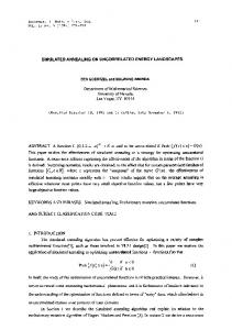
FIGURE II COMPARISON OF CPU TIME
�
�
�
�
�
�
�
�
II 0 0 0 0 0 0 0 0 0 0 0 0 0 0 0 0 0 0 0 0 0 0 0 0
�
III 0 0 0 0 0 0 0 0 0 0 0 0 0 0 0 0 0 0 0 0 0 0 0 0
�
�
�
�
IV 0 0 1 1 0 0 0 0 0 1 1 1 1 1 0 0 0 0 1 1 0 0 0 0
�
�
V 0 0 1 1 0 0 0 0 0 0 0 1 1 0 0 0 0 0 0 0 0 0 0 0
�
�
VI 0 0 0 0 0 0 0 0 0 0 0 0 0 0 0 0 0 0 0 0 0 0 0 0
�
�
VII 0 0 0 0 1 1 0 0 0 0 1 1 0 0 0 0 0 0 0 0 0 0 0 0
�
�
�
CPU Time in Seconds
I 0 0 0 0 0 0 0 0 0 0 0 0 0 0 0 0 0 0 0 0 0 0 0 0
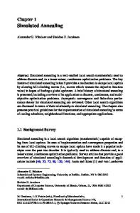
FIGURE III GRAPH BETWEEN NO. OF UNITS WITH TIME
�
6 4 2 0
C. Results Comparisons
0
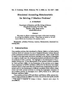
The cost and CPU time comparisons with Simulated Annealing method [10] are shown in Table VII. And the cost and CPU time comparisons with different methods are shown in Figure I and II. TABLE VII COMPARISONS OF RESULTS
Simulated Annealing Refined Simulated Annealing
RSA
Method
Figure III shows the graph between numbers of units should run during the number of hours.
Rs.12351764.000000
Method
80 70 60 50 40 30 20 10 0 SA
No. of Units
�
Total Cost (Rs.) 14606528.000000
CPU Time (Sec.) 80 75
12351764.000000
FIGURE 1 COMPARISON OF COSTS
200 Costs in Lakhs
�
Hour 1 2 3 4 5 6 7 8 9 10 11 12 13 14 15 16 17 18 19 20 21 22 23 24
150 100 50 0 SA
RSA Method
0-7803-7278-6/02/$10.00 ©2002 IEEE
4
8
12
16
20
24
Time (Hrs)
VII. CONCLUSION In this paper we considered the Unit Commitment Problem. The problem is highly combinatorial. Even moderate size problems are being solved with great difficulty. This paper presents a Refined Simulated Annealing Algorithm for solving the problem. The current Refined Simulated Annealing implementation has some advantage over that presented in. Our Refined Simulated Annealing provides a methodology for determining the initial control parameter (temperature and demand) at which all trail solutions are accepted. Moreover, temperature decrement is governed using statistics generated during the search (Polynomial-Time cooling schedule). Finally, new rules for generating feasible solutions are introduced, which results in considerable CPU time saving. Employing sophisticated tools in a Refined Simulated Annealing could lead to new unexplored solutions to the problem, which could result in better quality solutions. Further work in this area may be in parallel processing of the Simulated Annealing where each Markov Chain is processed by several processors, thus reducing the computation time or allowing for larger chains.
VIII. LIST OF SYMBOLS A i , B i ,C i ~ the cost function parameters of unit i (Rs./MWhr2.,Rs./MWhr.,Rs./ hr.) Cp ~ control parameter of the cooling schedule. Ckp ~ control parameter value at iteration k. F it (P it ) ~ production cost of unit i at a time t (Rs.hr.) FT ~ total operating cost over the scheduled horizon Fki ~ total operating cost for a current solution i at iteration k. N ~ number of available generating units P it ~ output power from unit i at time t (MW) Pki ~ output power from all units for a current solution i at iteration k. P min i ~ unit i minimum generation limit ( MW) P max i ~ unit i maximum generation limit ( MW) PD t ~ system peak demand at hour t (MW) R t ~ system reserve at hour t ( MW) S it ~ start up cost of unit i at hour t T~ scheduled time horizon ( 24 hrs. ) T up i ~ unit i minimum up time T down i ~ unit i minimum down time T on i ~ duration for which unit i is continuously ON T off i ~ duration for which unit i is continuously OFF T shut i ~ instant of shut down of a unit i T start i ~ instant of start up of a unit i U(0,1) ~ uniform distribution with parameters 0 & 1 UD(a,b) ~ discrete uniform distribution with parameters a and b Uit ~ unit i status at hour t = 1 ( if unit is ON) = 0 ( if unit is OFF) U k i ~ unit status matrix for a current solution i at iteration k V it ~ unit i start up / shut down status at hour t =1 if the unit is started at hour t and 0 otherwise. V k i ~ unit start up /shut down matrix for a current solution i at iteration k.
[6]
[7]
[8]
[9]
[10]
[11]
[12]
[13]
[14]
[15]
[16] IX. REFERENCES [1]
[2]
[3]
[4]
[5]
Wood. A.J. and Wollenberg. B.F.: ‘ Power Generation, Operation and Control ‘ John Wiley and Sons Ltd.1984. Pang.C.K., and Chen.H.C.: ’Optimal Short-term thermal unit commitment’, IEEE Trans.,1976, PAS95, pp.1336-1341. Hsu.Y.Y., SU, C.C.Liang,C.C.Lin.C.J. and Huang.C.T.: ’Dynamic security constrained multi-area unit commitment’, IEEE Trans. 1991, PWRS-6, pp.1049-1055. Misra.N., and Baghzouz.Y.: ’Implementation of the unit commitment problem on super computers’, IEEE Trans. 1994, PWRS-9, pp.305-310. Nieva,R., Inda.A., and Guillen.I.: ’Lagrangian reduction of search range for large scale unit
0-7803-7278-6/02/$10.00 ©2002 IEEE
commitment’, IEEE Trans. 1987, PWRS-2, pp.465473. Wang.S.J., Shahidehpour.S.M., Kirschen.D.S., Mokhtar.I.S., and Irisarri.G.D.: ‘Short – term generation scheduling with transmission and environmental constraints using an augmented Lagrangian relaxation’, IEEE Trans. 1995, PWRS-10, pp.1294-1301. Peterson.W.L., and Brammer.S.R.: ‘Crew constraints in Lagrangian relaxation unit commitment’, Proccedings of IEEE South – eastern’95, Visulalize the Future, 1995, pp.381-384. M.P.Kennedy and L.O.Chua, ‘Unifying the tank and hopfield linear programming circuit and the canonical non-linear programming circuit of chua and lin’, IEEE Trans. 1987, CAS-34, pp.210-214. Glover, F.: ‘Future paths for integer programming sand links to artificial intelligence ‘, COR-13 (5), 1986, pp.533-549. Zhuang.F., and Galiana, F.D.: ‘Unit commitment by simulated annealing’, IEEE Trans. 1990, PAS-5, pp.311-318. Mantawy.A.H., Abdel-Magid, Y.L., and Selim, S.Z.: ‘A simulated annealing algorithm for unit commitment ‘, IEEE Trans. 1998, PAS-13, pp.197-204. M.Djukanovic, B.Babic, B.Milosevic, D.Sobajic and Y.-H.Pao, ‘Fuzzy linear programming based optimal fuel scheduling incorporating blending / transloading facilities’, IEEE Trans. 1996, PAS-11, pp.1017-1023. General Introduction to Neural Computing, " Artificial Neural Networks in Power Systems - Part I ", Power Engg. Journal, Vol.11, No.3, June 1997. Philip.D.Wasserman (1989),"Neural Computing Theory and Practice ", Newyork, Van Nostrand , Reinhold. Alianna Maren , Craig Harston and Robert Pap(1990)"Handbook of Neural Computing Applications" ,USA Harcourt, Brace ,Jovanovich Goldberg, D.E, “Genetic Algorithms in Search Optimization and Machine Learning”, (Addison Wesley Publishing Company, Inc. Reading 1989).