An evaluation of the simulated annealing algorithm for solving the ...

2500

An evaluation of the simulated annealing algorithm for solving the area-restricted harvestscheduling model against optimal benchmarks Kevin A. Crowe and J.D. Nelson

Abstract: A common approach for incorporating opening constraints into harvest scheduling is through the arearestricted model. This model is used to select which stands to include in each opening while simultaneously determining an optimal harvest schedule over multiple time periods. In this paper we use optimal benchmarks from a range of harvest scheduling problem instances to test a metaheuristic algorithm, simulated annealing, that is commonly used to solve these problems. Performance of the simulated annealing algorithm was assessed over a range of problem attributes such as the number of forest polygons, age-class distribution, and opening size. In total, 29 problem instances were used, ranging in size from 1269 to 36 270 binary decision variables. Overall, the mean objective function values found with simulated annealing ranged from approximately 87% to 99% of the optima after 30 min of computing time, and a moderate downward trend of the relationship between problem size and solution quality was observed. Résumé : Le modèle de restriction de surface est une approche fréquemment utilisée pour contraindre la taille des aires de coupe dans la préparation d’un calendrier de récolte. Ce modèle est utilisé pour sélectionner les peuplements qui composent chacune des aires de coupe et établir un calendrier optimal de récolte englobant plusieurs périodes. Dans cet article, les auteurs utilisent des points de références optimaux qui proviennent de calendriers de récolte représentant plusieurs situations dans le but de tester un algorithme métaheuristique couramment utilisé pour résoudre de tels problèmes, le recuit simulé. La performance de l’algorithme du recuit simulé a été évaluée pour une gamme d’attributs du problème tels que le nombre de polygones forestiers, la distribution des classes d’âge et la dimension des aires de coupe. Au total, 29 variations du problème, variant en taille de 1 269 à 36 270 variables décisionnelles binaires, ont été utilisées. Dans l’ensemble, la moyenne des valeurs de la fonction objective trouvée avec le recuit simulé, atteignait approximativement 87 % à 99 % de l’optimum après 30 min de temps de calcul. Une tendance modérée à la baisse de la relation entre la taille du problème et la qualité de la solution a été observée. [Traduit par la Rédaction]

Crowe and Nelson

Introduction In forest management it is common for the size of harvest openings to be regulated and for harvest delays to be placed on all stands adjacent to these openings. Historically, these regulations were used to prescribe small, uniform openings dispersed across the forest, and now they are routinely used to control opening size distributions based on natural disturbances. The problem of determining which stands to include in each opening while simultaneously determining a harvest schedule over multiple time periods is a typical tactical forest planning exercise, and there is an enormous number of possible solutions. This approach is known as the arearestricted model (ARM). In the ARM, the boundaries of all potential cutblocks are not predefined. Instead, polygons Received 20 January 2005. Accepted 15 June 2005. Published on the NRC Research Press Web site at http://cjfr.nrc.ca on 2 November 2005. K.A. Crowe.1 Faculty of Forestry, Lakehead University, 955 Oliver Road, Thunder Bay, ON P7B 5E1, Canada. J.D. Nelson. Department of Forest Resources Management, The University of British Columbia, 2045 - 2424 Main Mall, Vancouver, BC V6T 1Z4, Canada. 1

Corresponding author (e-mail: [email protected]).

Can. J. For. Res. 35: 2500–2509 (2005)

2509

may be aggregated to form cutblocks during the search for an optimal solution. The limit of this aggregation is defined by the maximum allowable opening area. Opening size regulations are an operational reality, but the challenges they pose to modeling and solving the harvest-scheduling problem have not been fully addressed. One such challenge is the evaluation of neighbourhoodsearch metaheuristic algorithms, now widely used for solving the harvest-scheduling problem with constraints on opening sizes. Metaheuristic algorithms have been extensively used because the harvest-scheduling problem with opening size constraints is a binary integer programming problem, i.e., for a solution to be spatially explicit, a given stand must be either harvested or not harvested in a given period. Most large integer programming problems are notoriously difficult to solve using exact algorithms. Partial enumeration by exact algorithms often has a slow convergence rate, and only small or medium-sized problems have thus far been solved to optimality (Crowe et al. 2003). Since many practical harvest-scheduling problems are large, metaheuristics have been used instead of exact algorithms. One problem with metaheuristic algorithms is that they produce approximately optimal solutions, i.e., they neither guarantee optimality nor provide any indication of how close their solutions are to being optimal (Reeves 1993). Clearly,

doi: 10.1139/X05-139

© 2005 NRC Canada

Crowe and Nelson

it is important to form some estimate of how close the objective function of a metaheuristic solution is to optimality for a given type of problem (Wolsey 1998). The objective of this paper is to use an empirical approach to evaluate the ability of a simple implementation of a metaheuristic algorithm, simulated annealing, to solve a variety of instances of the harvest-scheduling problem modeled with opening size restrictions. Each of these instances has been solved optimally using the formulation methods discussed in Crowe et al. (2003), and therefore optimal benchmarks are to be used in the evaluation. By testing a metaheuristic across a range of instances, the objective is to gain some idea on how well it performs in general, and in what circumstances it does relatively well or relatively poorly. By using a simple implementation of the simulated annealing algorithm, the intention is to provide an empirical worst-case analysis of the potential of metaheuristic search algorithms in solving the area-restricted model to identify problem characteristics most in need of innovative advances. The outline of this paper is as follows: first, we review the literature relevant to testing heuristic performance along with recent research on solving the area-restricted model. Second, we present the formulation of the area-restricted harvest-scheduling problem. Third, we describe the benchmark problem instances used in this study. Fourth, we introduce the simulated annealing algorithm used to solve these problem instances. Fifth, we present results, comparing the objective functions of solutions produced using simulated annealing with those of optimal solutions. Finally, we discuss these results and conclude with suggestions on further research.

Literature review Reeves (1993) identifies three methods by which heuristic performance can be evaluated: (1) analytical methods, (2) statistical inference, and (3) empirical testing. With the analytical method, it is possible to analyze the operations of some heuristics such that their worst case or average performance on a problem can be proven. For example, it has been proven that a particular heuristic for the traveling salesman problem will always produce a solution not more than 50% longer than the optimal (Johnson and Papadimitriou 1985). Such proofs, though mathematically challenging, are of limited practical use unless the performance bounds can be made tight. Also, local search methods (on which the metaheuristics of simulated annealing and tabu search are based), because of the random elements in their operation, have been shown to have no performance guarantee for the traveling salesman problem (Reeves 1993). With the analytic method, it also possible to obtain a bound for a particular problem instance by using some form of relaxation of the problem, for example, a relaxation of integer constraints. Again, the usefulness of this approach for evaluating heuristic performance depends on how tight the gap is between the value of the bound and the heuristic solution. Statistical inference has also been used to estimate the performance of a heuristic. This approach was developed by Golden and Alt (1979) and is based on the statistical theory of extreme values (Fisher and Tippett 1928). Golden and Alt (1979) argue that each time we apply a heuristic to a

2501

minimization problem, we implicitly sample a large number, m, of possible solutions among which we find the minimum objective function value, vi. As m approaches infinity, the distribution of vi approaches the Weibull distribution. Given n independent solutions obtained in this way, it is possible to find a point estimate for the overall minimum and a confidence interval. Golden and Alt (1979) strongly supported the validity of this approach through extensive testing on the traveling salesman problem. Notwithstanding their efforts, according to Reeves (1993) there are few other reported applications of this approach in the literature. Among the few, Boston and Bettinger (1999) tested this approach on the 0–1 harvest-scheduling problem and concluded that extremevalue statistics provide unreliable estimates of the optimal objective function value and that the quality of the estimate is strongly dependent on the quality of solutions generated by the heuristic procedure. The empirical approach to testing a heuristic involves comparing its performance with that of existing techniques on a set of benchmarks. Since benchmarks represent only a small fraction of the possible population of instances, they should be sufficiently representative of real problems. Testing a heuristic across a range of problem instances facilitates evaluation of how well the heuristic performs in general and under what conditions it performs relatively well or poorly. Factors commonly discussed are the influence of problem size, solution quality, solution variance, and computational costs (Reeves 1993). In research on the integer harvest-scheduling problem, some evaluation of metaheuristic methods has occurred. For example, Nelson and Brodie (1990) used Monte Carlo integer programming to solve a three-period problem with 291 binary decision variables to within 10% of the known optimal. Murray and Church (1995) compared tabu search, simulated annealing, and hill climbing on the same data set used by Nelson and Brodie; the simulated annealing metaheuristic produced solutions averaging within 8% of the objective function of the optimal, and tabu search produced solutions averaging within 6.3%. On a larger data set, consisting of 1293 binary decision variables, Murray and Church (1995) found that simulated annealing solutions averaged within 11.8% and tabu search solutions averaged within 4.4% of the known optima. Weintraub et al. (1995) interfaced metaheuristic decision rules with a continuous linear programming (LP) solver to produce an integer solution averaging within 6.4% of the known optimal for a transportation and scheduling problem comprising 191 integer decision variables. Boston and Bettinger (1999) compared tabu search and simulated annealing, on four problem instances ranging is size from 3000 to 5000 decision variables. The simulated annealing algorithm produced solutions within 3.4%, 1.9%, 0.2%, and 3.5% of the known optima of the four problems, while the tabu search produced solutions within 6.3%, 2.8%, 0.0%, and 4.3%. In all of the above comparisons, the type of harvestscheduling model evaluated was the unit-restricted model (URM). In the URM, the boundaries of all potential harvest openings are predefined, i.e., the boundary of each polygon in a problem instance equals the boundary of each potential cutblock (i.e., contiguous area of harvested forest). The other modeling approach to controlling opening sizes in harvest © 2005 NRC Canada

2502

schedules is the ARM, in which the boundaries of all potential cutblocks are not predefined, and this model has not been fully evaluated. It is important that an evaluation of metaheuristic algorithms used to solve the ARM be made, for two reasons: (1) the ARM is, arguably, a more suitable model of the harvest-scheduling problem than the URM; and (2) the ARM is potentially more difficult to solve. We discuss each reason in detail. First, the ARM has several advantages over the URM. For example, it has been observed (Walters et al. 1999; Richards and Gunn 2000) that in the ARM the configuration of cutblocks emerges in the context of an optimal flow of timber, and that the predefined cutblocks of the URM may underestimate the potential harvest flow through suboptimal cutblocks. Moreover, research indicates that poor block configuration can contribute to lower objective function values (Jamnick and Walters 1991). Murray and Weintraub (2002), using several methods by which to preaggregate polygons into cutblocks, demonstrate that the ARM consistently produces objective function values that are superior to those of the URM. Second, the ARM may be more difficult to solve than the URM. Our reasoning for this is that the number of feasible solutions to a given problem instance can be much greater when modeled as an ARM than as a URM. The degree to which this difficulty increases depends on the difference in area between the polygons and the maximum opening size restriction. For example, given an opening size restriction of 40 ha and an average polygon size of 5 ha, in one case, and an average polygon size of 15 ha in another case then, all other things being equal, the number of feasible combinations will be much greater in the former case than in the latter. The URM avoids this type of expansion of the solution space. Murray and Weintraub (2002), for example, rightly observe that the URM can provide a lower bound on problems modeled as an ARM. As mentioned above, in the case of the ARM, metaheuristic algorithms have not been fully evaluated, because formulations have only recently emerged for exact optimal solutions to the ARM (McDill et al. 2002; Crowe et al. 2003; Caro et al. 2003). McDill et al. (2002) solved problem instances up to 80 polygons over three periods, on a simulated forest designed to allow not more three polygons to aggregate within an allowed opening. Caro et al. (2003) evaluated a tabu search metaheuristic on six instances of a forest of 20 stands over two periods. Their metaheuristic solutions were within 1% of the optimal, but they noted that the instances were too small to evaluate the true merit of their metaheuristic. Caro et al. (2003) also used a case study of 574 stands over seven periods and found that their tabu search algorithm produced solutions within 8% of an LP upper bound. Crowe et al. (2003) evaluated exact formulations of the ARM on five forests ranging in size from 346 to 6093 polygons scheduled over three periods. These provide solid benchmarks by which to evaluate metaheuristic solutions to the ARM.

Problem definition and model Formulations of the ARM are tested by scheduling harvest

Can. J. For. Res. Vol. 35, 2005

activities over three 20-year periods in a forest with an 80-year rotation period. The objective is to maximize net present value of the harvest activities, where value is measured at $100/m3, discounted from the middle of each planning period at 4%. Harvest activities are restricted to clear-cutting or doing nothing. The constraints in this problem are (1) A limit on interperiod harvest volume fluctuations of plus or minus 10%. (2) A limit on opening size of 40 ha, with a one-period restriction on harvesting of all adjacent polygons (adjacency is defined as sharing a common boundary node). (3) A minimum harvest age of 80 years. (4) An ending-age constraint to ensure that the average age of the forest at the end of the planning horizon be at least 40 years (i.e., the average age of a forest regulated on an 80-year rotation). The formulation of the endingage constraint is from McDill and Braze (2000). The notation and mathematical formulation of the model are presented below: xit equals 1 if polygon i is harvested in period t = 1, 2, or 3; 0 otherwise Note that if polygon i has not been cut for the entire planning horizon, then xit = 1 when t = 0. This is done to implement the ending age constraint. vit is the volume of polygon i in period t (m3) rit is the discounted net revenue from harvesting polygon i in period t ($) ai is the area of polygon i (ha) Ht is the total volume harvested in period t (m3) eit is the ending age of polygon i if harvested in period t (ending age is measured in year 60) I is the set of all polygons in the forest Oit is the set of stands, including stand i, that are harvested during period t and are included in the same opening as stand i (i.e., contiguously connected to stand i) Omax is the maximum opening area for harvest blocks (ha) The objective function is to maximize the net present revenue: I

[1]

maximize

3

∑ ∑ ritxit i =1 t =1

subject to (1) each polygon may be assigned not more than one prescription over the planning horizon: 3

[2]

∑ xit = 1

∀i = 1, K, I

t= 0

(2) accounting variables defining the total volume harvested in each period: I

[3]

∑ vit xit − Ht = 0

∀t = 1, K, 3

i =1

(3) limit on total area of polygons aggregating into harvest blocks for each period: [4]

∑ xita i ≤ Omax

∀i ∈ I;

t = 1, K, 3

i ∈Oit

© 2005 NRC Canada

Crowe and Nelson

2503 Table 1. Spatial attributes of the seven benchmark forests. Polygon area (ha)

Polygon adjacencies

Forest

Total area (ha)

No. of polygons

Min.

Max.

Mean

Min.a

Max.

Mean

Gavin Hardwicke Naka Stafford Kootenay I Kootenay II Kootenay III

6 193 6 948 10 934 10 421 38 441 71 257 118 535

346 423 785 1 008 3 256 6 093 12 090

1.1 3.0 0.06 2.0 6.0 6.0 6.0

43.0 42.0 43.0 20.0 38.0 38.0 39.5

17.9 16.4 13.9 10.3 11.8 11.7 9.8

1 2 1 0 0 0 0

16 10 14 12 15 15 15

5.8 6.1 5.2 4.3 5.6 5.2 5.2

a

A few isolated polygons in Kootenay I, II, and III, and Stafford have no neighbours.

(5) interperiod harvest volumes may fluctuate at most by 10%: [5]

− 0.9Ht + Ht +1 ≥ 0

t = 1, 2

[6]

−1.1Ht + Ht +1 ≤ 0

t = 1, 2

(4) average polygon age of total forest area must be at least 40 years at the end of planning horizon (year 60): I

[7]

Polygons eligible for harvest in period 1

Range of uniform distribution of ages

50% 75% 100%

10–150 years 40–200 years 80–200 years

3

∑ ∑ (eit − 40)a ixit ≥ 0 i =1 t = 0

(5) the decision variables are binary: [8]

Table 2. Three age distributions randomly assigned to each forest.

x it ∈ {0, 1}

∀i = 1, K, I;

t = 0, K,3

Description of benchmarks Spatial data from seven forests in British Columbia were used in this study. Table 1 summarizes the spatial attributes of these forests, including the size of polygons and the mean number of adjacencies per polygon. Polygons in the smaller forests — Gavin, Hardwicke, and Naka — were manually drawn by forest engineers, while the polygons of Stafford and Kootenay were formed by GIS overlays. The forest of Kootenay I is a subset of polygons extracted from the larger forest, Kootenay II, which is similarly a subset of Kootenay III. Polygons ranged in size from 0.06 to 43 ha (a few polygons marginally greater than the 40-ha opening limit are allowed to be harvested by themselves). We were also interested in testing different age-class distributions for each forest. McDill and Braze (2000) found a strong correlation between the initial age-class distribution of a forest and the difficulty of solving the URM using a branch and bound algorithm, namely that problems with a higher proportion of old-growth forest area are, in general, more difficult to solve than others. For this reason, we assigned three age-class distributions to each forest to test the formulations on each. The age-class distributions are based on the percentage of polygons eligible, by age, for harvest in the first period. The three distributions tested are 100%, 75%, and 50%. Table 2 summarizes the uniform age distributions assigned to each forest using a random number generator. In addition to the effect of different age-class distributions, we also wished to explore the effects of different maximum opening size limits. Increasing the opening size limit

allows for more possible combinations of polygons to aggregate into a feasible opening, thereby increasing the number of possible solutions. For this reason, we tested four different opening size limits on the Stafford forest: 20, 30, 40, and 50 ha. The methods used to compute optimal solutions for these forests are described fully in Crowe et al. (2003).

Description of the simulated annealing algorithm The simulated annealing algorithm used to solve the harvest-scheduling problem is similar to that designed and illustrated by Boston and Bettinger (1999), except for the choice of parameters: namely, the initial solution, the initial temperature, the reduction factor, the definition of a neighbourhood, and the number of iterations at a given temperature. To illustrate the context of these parameter choices, we first present a concise outline (Wolsey 1998) of the simulated annealing metaheuristic. (1) Get an initial solution, S. (2) Get an initial temperature, T, and a reduction factor, r, with 0 < r < 1. (3) While T is not frozen, (i) perform the following loop nrep times: pick a random neighbour S′ of S; if S′ is feasible, let delta = f(S′) – f(S), if delta ≥ 0, set S = S′, if delta < 0, set S = S′ with probability e–delta/T; (ii) Set T = rT. (4) Return best solution. We defined a neighbour of S to be any solution arising from the following operation: (1) Randomly select any binary decision variable, xij (where i = 1, ÿ, I; and t = 1, ÿ, 3) from the current solution, S (where xij = 1 if polygon i is harvested in period j; 0 otherwise). (2) If xij = 0, let xij = 1. (3) If if xij = 1, let xij = 0. © 2005 NRC Canada

2504

(4) If this permuted solution is feasible, then it is a neighbour, S′. Note that only feasible solutions can be accepted in this algorithm. The manner of defining a neighbour of S was based on the idea that small neighbourhoods are preferable to large complex ones (Reeves 1993). We should note that the choice of a neighbourhood structure can itself be the subject of some experimentation, and that Bettinger et al. (1999) have initiated such research for a tactical planning problem. The choice of an initial feasible solution followed naturally from this choice of a neighbourhood: first, we set all xij’s, for all positive periods, equal to zero; second, we temporarily altered the constraint limiting interperiod harvest fluctuations. This constraint was altered such that the volume harvested in period t cannot differ from the volume harvested in periods t – 1 or t + 1 by more than a fixed value. This value equals the volume contained in the stand with the highest volume for a given problem instance. Finally, we ran the model for 50 000 iterations with a zero probability of accepting inferior solutions. This method produced feasible initial solutions of random quality. The solutions were feasible because after 50 000 iterations, 10% of the average periodic volume harvested greatly exceeds the volume of the polygon with the greatest volume. The parameters requiring experimentation were r, T, and nrep. For each problem instance, an experiment was designed to find the best values for these parameters within a reasonable period of time, which was complicated by the fact that the annealing algorithm is randomized, and therefore results of a single run may not be typical. To simplify the execution of the experiment, we set r = 0.99 as a constant. This choice was supported by the literature on simulated annealing, which indicates that most reported successes use values between 0.8 and 0.99 with a bias to the higher end of the range (Reeves 1993). The value of an initial experimental temperature, T, was determined for each problem instance by setting r = 1.0, iteratively running the algorithm, and raising T, until all feasible solution changes were accepted with at least 95% probability. The intention here was to find a value for T allowing an almost free exchange of neighbouring solutions so that the final solution would be independent of earlier solutions. Finding a value for nrep was complicated by our intention to evaluate the search algorithm’s effectiveness after fixed periods of processing time. This time constraint requires, for example, that a short run must cool more rapidly than a long run. The fixed processing time constraint was imposed by first estimating the mean number of iterations per unit time for a given problem instance and then selecting a value for N, the number of iterations after which the search algorithm stops. In other words, the stopping criterion used in the algorithm is a fixed number of iterations. The value of nrep governs the number of repetitions at each temperature; therefore, given a fixed number of iterations for the entire run, N, we had to ensure not only that the probability of accepting inferior solutions became very low by the time N iterations had passed, but also that the algorithm did not proceed too quickly to a state not accepting inferior solutions, thereby wasting time trapped in a local optimum. We therefore tested different values for nrep, beginning with a


value of nrep equal the number of binary decision variables in each problem instance, and then iteratively doubling the value of nrep and rerunning the algorithm until convergence at a sufficiently cool temperature occurred, i.e., until the probability of accepting an inferior solution became extremely small. In our testing, after approximately 200 000 iterations occurred without the acceptance of an inferior solution, we considered this state sufficiently cool. Our intention in adjusting nrep in this way was to avoid wasting too much search time in a cooled state, i.e., trapped in a local optima. The cooled state is a function not only of temperature, but also of the difference between candidate objective function values. The harvest-scheduling model using the simulated annealing algorithm was encoded in the C programming language, using Microsoft Visual C++ version 6.0. Optimal solutions were computed using CPLEX 8.1. All models were solved using a 2.4 GHz Pentium 4 CPU, with 1.5 gigabytes of RAM, and a Windows XP operating system.

Results The solution qualities and variances for all problem instances solved using the simulated annealing algorithm are presented in Table 3. In Table 3, mean solution quality refers to the mean objective function value of the solutions produced by simulated annealing for each problem instance divided by the optimal objective function value. For each problem instance, a unique set of parameters was devised, and for each solution generated for each problem instance, a unique initial solution was randomly generated and used. Gap variance refers to the standard deviation of those solutions divided by the optimal objective function value. We use this measure because it describes not only how widely values are dispersed around the mean metaheuristic objective function value, but also because it describes this value in terms of the variance in the gap between the metaheuristic and optimal solution values. Each of the run times in Tables 3 and 4 resulted from the adjustment of cooling parameters, as described in Methods. Each mean requiring 3 min of computing time is based on a sample of 30 solutions, while the means requiring 30 min are based on a sample of 15 solutions. Five 3-h runs were executed for any problem yielding a mean objective function value of less than 90% of the optimal on a 30-min run; results are presented in Table 4. The simulated annealing algorithm evaluated, on average, 136 million solution permutations per minute. Results from the Kootenay III forest are not included in Table 3 for the instance where 100% of the stands are initially eligible. This is because no optimal solution was found — the branch and bound solution tree required more memory than was available. The objective in testing the simulated annealing algorithm was to observe how well it performs in general and under what circumstances it will do relatively poorly. This objective will guide analysis of the results. First, in general, the mean solution produced by the simulated annealing algorithm for all 29 instances, using 30 min of computing time, ranged from approximately 87% to 99% of the optima, and the mean gap variance (as defined above) ranged from about 0.1% to 2.3%. © 2005 NRC Canada

Crowe and Nelson

2505 Table 3. Solution quality and gap variance from applying simulated annealing to benchmark instances. 3-min runs

Forest Gavin

Hardwicke

Naka

Stafford 20 ha

Stafford 30 ha

Stafford 40 ha

Stafford 50 ha

Kootenay I

Kootenay II

Kootenay III

Mean solution quality (%)

Gap variance (%)


Gap variance (%)

50 75 100 50 75 100 50 75 100 50 75 100 50 75 100 50 75 100 50 75 100 50 75 100 50 75 100 50 75

94.2 95.4 94.9 98.0 98.3 98.6 89.3 90.5 91.8 96.5 95.2 97.1 98.4 98.5 98.7 98.8 98.4 98.6 99.1 98.4 98.6 90.7 92.3 93.8 87.1 87.3 88.5 88.5 90.81

0.68 0.73 0.63 0.51 0.42 0.72 0.11 0.32 0.29 0.35 0.60 0.37 0.16 0.07 0.04 0.05 0.04 0.02 0.05 0.03 0.08 0.32 2.06 1.26 1.14 2.56 1.72 0.27 1.20

94.5 95.5 95.0 98.0 98.4 98.8 91.4 92.5 93.4 97.1 96.1 97.7 98.4 98.5 98.7 98.8 98.5 98.6 99.1 98.4 98.7 91.0 92.5 93.9 87.1 87.4 88.6 88.5 90.8

0.70 0.20 0.82 0.55 0.58 0.42 0.49 0.32 0.34 0.26 0.61 0.36 0.18 0.09 0.05 0.06 0.04 0.04 0.06 0.03 0.05 0.13 1.07 0.98 1.46 2.31 1.57 0.17 0.78

Table 4. Solution quality and gap variance results from 3-h runs using the simulated annealing algorithm. Forest Kootenay II

Kootenay III

30-min runs

Stands eligible for harvest (%)

Stands harvestable in period 1 (%)


Gap variance (%)

50 75 100 50 75

87.6 87.9 88.8 88.9 91.1

1.29 1.31 1.57 0.17 0.78

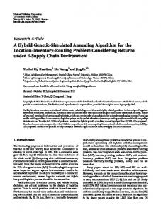
Second, in particular, the effects of attributes of particular problem instances that interested us were (i) the number of decision variables; (ii) the percentage of stands initially eligible for harvest; and (iii) the ratio between the mean polygon area and the maximum opening area. We examine these separately. The relation between the number of decision variables and the solution quality, for each of the 30-min runs are presented in Fig. 1. Figure 1 indicates that there is a downward trend between problem size and the quality of solutions produced by the simulated annealing algorithm. The problem instances that

most weaken this trend are from the Naka and Kootenay II forests, and they comprised 2355 and 18 279 binary decision variables, respectively. Each of these forests yields solutions relatively inferior to those of larger forests. Clearly there is an attribute, or attributes, other than problem size also influencing the algorithm’s search for better solutions. We considered whether the relatively poor solution qualities of Naka and Kootenay II might have arisen from either (i) the chance that the particular random assignment of ages might have made the problem instance difficult to optimize using neighbourhood search; or (ii) the particular spatial arrangement of the polygons in these forests. Looking at Fig. 1 and noting that variance in solution quality among the seven forests is greater than the variance within the three different age-classes randomly assigned to each forest, we were inclined to pursue (ii) as a possible venue for explanation. Unfortunately, the spatial attributes of the forests, presented in Table 1, reveal no attribute by which to differentiate both Naka and Kootenay II from the other forests. The influence of the number of binary decision variables is more pronounced, however, when we compare the progress made on solution quality when moving from the 3-min to 30-min runs. Here the progress made on the smaller Naka © 2005 NRC Canada

2506


Fig. 1. Relation between mean solution quality and number of binary decision variables (Note: number of decision variables equals number of polygons times three periods. We do not count xit, when t = 0, as a true decision variable, for it essentially functions as an accounting variable). 50% eligible

75% eligible

100% eligible

100

Solution Quality (% Optimum)

98

Stafford

96

Gavin 94

Naka

92

Kootenay I

90

Kootenay III Kootenay II

88 86 0

5 000

10 000

15 000

20 000

25 000

30 000

35 000

40 000

No. of Binary Decision Variables

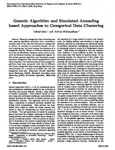
problems produced a mean improvement of 1.90%, while on the much larger forests of Kootenay II and III, mean progress was 0.20% and 0.07%, respectively. In fact, the solutions to the Kootenay II and III forests benefitted very little from the additional 3 h of computing time (Table 4), improving upon the 30-min solution quality by a mean of 0.47% and 0.35%, respectively. Increased computing time had little effect on gap variance. To assess changes in gap variance, we arbitrarily defined a change to occur if the gap variance increased or decreased by more than ±0.05%. When moving from 3-min to 30-min runs, 16 were unchanged, 3 increased, and 10 declined (total of 29 gap variances). Of the seven solutions with 30-min and 3-h runs, five gap variances were unchanged, and two decreased. The small gap variances indicate the solutions are tightly grouped around their respective means. Apart from the effect of the number of decision variables, we were also interested in the effect of the mean polygon size on the solution quality. In the Introduction, we reasoned that the smaller the mean polygon area relative to the maximum opening area, the more feasible combinations there would be, the larger the solution space would be, and therefore the more difficult it would be to find near-optimal solutions. This speculation is supported by the results of Crowe et al. (2003), who, in solving the ARM with increasing opening size constraints using the branch and bound algorithm, found that instances with larger opening constraints consistently required more computing time, i.e., they were more difficult to solve. Table 3 indicates that the simulated annealing algorithm is not similarly affected by increasing opening size constraints. For example, in the Stafford forest, the solution quality improves from a 20-ha opening to a 50-ha opening. Figure 2 indicates that there is no apparent trend between solution quality and the ratio of mean polygon area to maximum opening area for all of the instances solved.

Finally, we were interested in the effect of initial age-class distribution on solution quality. The results in Table 3 reveal that six of the seven forests yielded their worst mean solution qualities to the youngest forest (50% initially eligible) while five of the seven forests yielded their best mean solution qualities to the oldest forests. This indicates that problems with fewer eligible stands are more difficult to optimize for a metaheuristic than problems where more stands are eligible. These findings are contrary to those for the branch and bound algorithm, where older forests are more difficult to optimize.

Discussion The results uncover several trends worthy of discussion. The first, and perhaps most important trend, is that problem size does moderately affect the ability of the simulated annealing algorithm to find near-optimal solutions. A weak trend was observed between larger problem instances and poorer solution qualities; but the decline in quality was not steep. The simulated annealing algorithm produced excellent results, which were, on average, within 5% of the optima over the range of instances tested. Of course, the number and size of the instances solved in this research cannot allow us to generalize this trend with certainty, but the results can provide some confidence to practitioners currently using neighbourhoodsearch metaheuristics to produce efficient tactical-level plans in forest management. Not all neighbourhood-search metaheuristics have been shown to cope equally well in finding near-optimal solutions as problem size increases (see Johnson and McGeoch (2002) for heuristic algorithms used on increasingly larger instances of the traveling salesman problem). A second interesting result provided by this research, especially from the Stafford forest, is that the ratio of the mean © 2005 NRC Canada

Crowe and Nelson

2507

Solution Quality (% Optimum)

Fig. 2. Relation between qualities of solutions produced by simulated annealing algorithm and the ratio of mean polygon area to maximum opening area. Results illustrated are from the 30-min runs, with different solutions for each of the three initial age-class distributions per forest.

100 98 96 94 92 90 88 86 0

0.1

0.2

0.3

0.4

0.5

0.6

Ratio of Mean Polygon Area to Maximum Opening size polygon area to the maximum opening area did not influence the quality of the best solution found by the metaheuristic. As noted earlier, the smaller this ratio is, the greater is the number of feasible solutions (other things being equal). We are therefore obliged to ask the following: why did problems with a smaller ratio not yield solutions of lower quality, given the expansion of the solution space? Our answer to this is complemented by reflection on another question raised by this research: namely, why is it that forests with 100% of the stands initially eligible for harvest yielded solutions of higher quality than forests with only 50% of the stands initially eligible? This question complements the first because, in both cases, problem instances with relatively more feasible solutions yield solutions that are of equal or higher quality than instances with relatively fewer feasible solutions. Why? The number of feasible solutions relative to the number of decision variables influences solution quality because it influences the neighbourhood search. For example, let S be a set of feasible solutions to a particular problem, and N(s) be the neighbourhood of a solution, s. In neighbourhood search, N(s) is defined as the set of solutions that can be obtained from s by performing a simple permutation operation on s. But not all such permutations on s produce a solution within the set N(s), because some of these permutations produce infeasible solutions. Hence, if there are, for example, more feasible solutions in problem A than in problem B, then, on average, each neighbourhood of each solution in A will have a greater number of members than each neighbourhood of each solution in B. This can have two major effects on the neighbourhood search in problems A versus B: (i) more time is lost in problem B than in problem A by producing infeasible solutions through a permutation operation, and more importantly (ii) the ability of the algorithm to diversify the search, i.e., enter new regions of the solution space, is hampered when neighbourhoods are smaller. Hertz and Widmer (2003), for example, have also observed the relative ineffectiveness of neighbourhood search in highly constrained problems where permutation operations rarely produce a feasible solution. To promote diversity in the search, they suggest relaxing some constraints and adding penalties to the objective

Gavin Hardwicke Naka Stafford 20 ha Stafford 30 ha Stafford 40 ha Stafford 50 ha Kootenay I Kootenay II Kootenay III

function. In our evaluation of the metaheuristic solutions of the ARM, penalty functions were not used because the model solved by the branch and bound algorithm neither required nor used penalty functions; therefore an informative comparison of objective function values reached using the two algorithms would have been misleading had these objective functions been different. Another point to discuss concerns the relation between problem formulation used in this research and the relative success of the simulated annealing algorithm in solving instances of this formulation. What, for example, might the effect have been on the search algorithm’s success had we added more constraints to the formulation? Here we can only speculate that the effects would have been mixed and unpredictable, for several reasons. On the one hand, by adding more constraints to a problem, the solution space either remains the same, or becomes smaller, and a smaller solution space, other things being equal, tends to improve the metaheuristic algorithm’s chances of finding better solutions. On the other hand, by adding more constraints to a problem, the computational burden of calculating the effect of a given solution permutation increases, and this tends to slow down the progress of the search. For example, calculating the effect of a solution permutation on remnant old-growth patch constraints can be computationally costly (Liu et al. 2000). Finally, as Herz and Widmer (2003) note, when a problem becomes very heavily constrained and feasible solutions are hard to find through a permutation operation, then penalty functions are needed for the metaheuristic to diversify its search. This reformulation of the problem can therefore affect the benchmarking exercise, for the addition of penalty weights to a model formulation requires that the branch and bound algorithm solve such models in the benchmarking exercise, even though penalty functions are not needed by the branch and bound algorithm. In other words, the procedure of evaluating the metaheuristic must become biased — through model reformulation — to accommodate the metaheuristic’s weaknesses. A final point of discussion requires us to interpret the general results: a mean solution quality of almost 95%, gener© 2005 NRC Canada

2508

ally with very little variance. What does this mean for the future of research on metaheuristic applications to the ARM? Clearly, there is little room for improvement, given that this is a worst case analysis. Closing the gap on the final 5% between metaheuristic versus optimal solution quality may present itself as an interesting challenge to researchers; but what might be the practical merit of this? Efficient solutions produced by a symbolic model rarely translate into equivalent results in operational realities. Hence, for the tactical harvest-scheduling problem, the minor increases in net present value that might arise by improvements in metaheuristic planning algorithms may never materialize, given uncertainties in field data, growth and yield data, and estimates of harvested log grades and values. The results of this research therefore point in one direction for future relevant research on applying metaheuristic algorithms to the ARM: evaluating algorithms using much larger problems instances. There are several reasons for this. First, since there was a trend observed between problem size and solution quality, it would be useful to explore this further. Second, the results revealed that the simulated annealing algorithm, when applied to the larger problems (Kootenay II and III), made very little improvement to solution quality between 3-min and 3-h runs. This indicates that on very large problems, it can be much more challenging to explore truly different regions of the search space effectively. Improvements in search diversification strategies should therefore be evaluated in the context of larger problem instances. Finally, although the optimal benchmarks by which metaheuristic solutions to larger instances of the ARM are to be evaluated may not be computationally feasible, the research of Crowe et al. (2003) and Caro et al. (2003) indicates that LP relaxations of the ARM provide reasonable estimates of the upper bounds.

Conclusions The objective of this paper was to apply the simulated annealing algorithm to a variety of instances of the area-restricted harvest-scheduling model and to evaluate its approximately optimal solutions by comparison with optimal benchmarks. Of the 29 instances solved, the average deviation from the optima ranged from approximately 1% to 13%. Attributes of the problem, such as the number of decision variables, maximum opening size, and initial age-class distribution were examined for their effect on the metaheuristic’s ability to produce good solutions. A weak downward trend was observed on the relationship between solution quality and problem size. This research is significant because it constitutes the first evaluation of the ability of a metaheuristic algorithm to produce good quality solutions for the ARM. Given that the application of the simulated annealing algorithm required no innovation and was relatively simple to implement, the results constitute a worst-case analysis of the potential of the metaheuristic approach to this problem. The strong results produced by this worst-case analysis, coupled with a moderate downward trend on the relation between problem size and solution quality, suggest that future research on applying metaheuristics to the ARM use relatively large problem instances.


Acknowledgements This research was funded by a collaborative grant from the National Science and Engineering Research Council of Canada, the Social Science and Humanities Research Council of Canada, the Canadian Forest Service, and Canadian Forest Products Ltd., entitled “Exploring, Forecasting and Visualizing the Sustainability of Alternative Ecosystem Management Scenarios”.

References Bettinger, P., Boston, K., and Sessions, J. 1999. Intensifying a metaheuristic forest harvest scheduling search procedure with 2opt decision choices. Can. J. For. Res. 29: 1784–1792. Boston, K., and Bettinger, P. 1999. An analysis of Monte Carlo integer programming, simulated annealing, and tabu search metaheuristics for solving spatial harvest-scheduling problems. For. Sci. 45: 292–301. Caro, F., Constantino, M., Martins, I., and Weintraub, A. 2003. A 2-opt tabu search procedure for the multiperiod forest harvesting problem with adjacency, greenup, old growth, and even flow constraints. For. Sci. 49: 738–751. Crowe, K., Nelson, J., and Boyland, M. 2003. Solving the arearestricted harvest-scheduling problem using the branch and bound algorithm. Can. J. For. Res. 33: 1804–1814. Fisher, R., and Tippett, L. 1928. Limiting forms of the frequency distribution of the largest or smallest member of a sample. Proc. Camb. Philol. Soc. 24: 180–190. Golden, B.L., and Alt, F.B. 1979. Interval estimation of a global optimum for large combinatorial problems. Nav. Res. Log. Quart. 26: 69–77. Hertz, A., and Widmer, W. 2003. Guidelines for the use of metaheuristics in combinatorial optimization. Eur. J. Oper. Res. 151: 247–252. Jamnick, M.S., and Walters, K.R. 1991. Spatial and temporal allocation of stratum-based harvest schedules. Can. J. For. Res. 23: 402–413. Johnson, D., and McGeoch, L. 2002. Experimental analysis of metaheuristics for the symmetric traveling salesman problem. In The traveling salesman problem and its variations. Edited by G. Gutin and A. Punnen. Kluwer Academic Publishers, Dordecht, Netherlands. pp. 369–443. Johnson, D.S., and Papadimitriou, C.H. 1985. Performance guarantees for heuristics. Interfaces, 2: 145–180. Liu, G., Nelson, J., and Wardman, C. 2000. A target-oriented approach to forest ecosystem design — changing the rules of forest planning. Ecol. Model. 127: 269–281. McDill, M.E., and Braze, J. 2000. Comparing adjacency constraint formulations for randomly generated forest planning problems with four age-class distributions. For. Sci. 46: 423–436. McDill, M.E., Rebain, S.E., and Braze, J. 2002. Harvest scheduling with area-based adjacency constraints. For. Sci. 48: 631–642. Murray, A.T., and Church, R.L. 1995. Metaheuristic solution approaches to operational forest planning problems. OR Spektrum, 17: 193–203. Murray, A.T., and Weintraub, A. 2002. Scale and unit specification influences in harvest scheduling with maximum area restrictions. For. Sci. 48: 779–789. Nelson, J., and Brodie, J.D. 1990. Comparison of a random search algorithm and mixed integer programming for solving areabased forest plans. Can. J. For. Res. 20: 934–942. © 2005 NRC Canada

Crowe and Nelson Reeves, C.R. (Editor). 1993. Modern metaheuristic techniques for combinatorial problems. Blackwell Scientific Publications, Oxford, UK. Richards, E.W., and Gunn, E.A. 2000. A model and tabu search method to optimize polygon harvest and road construction schedules. For. Sci. 46: 188–203. Walters, K.R., Feunekes, H., Cogswell, A., and Cox, E. 1999. A forest planning system for solving spatial harvest-scheduling problems. In Canadian Operations Research Society National Conference, 7–9 June 1999, Windsor, Ont. Available from

2509 http://www.remsoft.com/case_studies.php [accessed December 2003]. Weintraub, A., Jones, G., Meacham, M., Magendzo A., and Malchuk, D. 1995. Metaheuristic procedures for solving mixedinteger harvest-scheduling transportation planning models. Can. J. For. Res. 25: 1618–1626. Wolsey, L.A. 1998. Integer programming. John Wiley and Sons Ltd., New York.

© 2005 NRC Canada