Mobile mapping systems (MMS) can capture dense point-clouds of urban scenes. For visualizing realistic scenes using point-clouds,. RGB colors have to be ...
ISPRS Annals of the Photogrammetry, Remote Sensing and Spatial Information Sciences, Volume III-1, 2016 XXIII ISPRS Congress, 12–19 July 2016, Prague, Czech Republic
REFINEMENT OF COLORED MOBILE MAPPING DATA USING INTENSITY IMAGES T. Yamakawa a , K. Fukano a ,R. Onodera a, H. Masuda a, * a Dept. of Mechanical Engineering and Intelligent Systems, The University of Electro-Communications, 1-5-1 Chofugaoka, Chofu, Tokyo, Japan - (tooru.yamakawa, kenta.fukano, ryo.onodera, h.masuda)@uec.ac.jp
Commission I, ICWG I/Va KEY WORDS: Point-Cloud, Mobile Mapping System, Reflection Intensity, Calibration, Edge Detection, Color Information
ABSTRACT: Mobile mapping systems (MMS) can capture dense point-clouds of urban scenes. For visualizing realistic scenes using point-clouds, RGB colors have to be added to point-clouds. To generate colored point-clouds in a post-process, each point is projected onto camera images and a RGB color is copied to the point at the projected position. However, incorrect colors are often added to point-clouds because of the misalignment of laser scanners, the calibration errors of cameras and laser scanners, or the failure of GPS acquisition. In this paper, we propose a new method to correct RGB colors of point-clouds captured by a MMS. In our method, RGB colors of a point-cloud are corrected by comparing intensity images and RGB images. However, since a MMS outputs sparse and anisotropic point-clouds, regular images cannot be obtained from intensities of points. Therefore, we convert a point-cloud into a mesh model and project triangle faces onto image space, on which regular lattices are defined. Then we extract edge features from intensity images and RGB images, and detect their correspondences. In our experiments, our method worked very well for correcting RGB colors of pointclouds captured by a MMS.
1. INTRODUCTION A mobile mapping system (MMS) can be used to capture pointclouds of urban scenes. A MMS is a vehicle on which laser scanners, digital cameras, GPS, and IMU are mounted (Figure 1). Laser scanners output point-clouds, which contain 3D coordinates, intensity values, and GPS times. Intensity values represent the strength of reflected laser beams, and GPS times indicate when points were captured. MMSs measure their positions by receiving GPS data. When MMSs fail to catch GPSs, they estimate the vehicle position using IMUs and odometers. Digital cameras on a MMS capture successive digital images of scenes while a vehicle moves. Since the original coordinates from a laser scanner are described on the scanner-centered coordinate system, they have to transformed to global coordinates, such as WGS84 coordinates, by using the vehicle positions. Positions of a vehicle are typically measured using GPSs, IMUs, and odometers. In this paper, we use the Mitsubishi MMS-X, as shown in Figure 1. In this system, the positions and attitudes of cameras and laser scanners are represented relative to the coordinate system defined on the vehicle. These data were calibrated by the MMS vendor and the calibration data were given to the users. When the software tool, which is bundled with the MMS, processes raw MMS data, it outputs 3D coordinates with intensity, the transformation matrices of cameras and laser scanners, and camera parameters.
In this paper, we implemented the pinhole camera model proposed by Zhang, et al. (Zhang, 2000), and projected each point on images. To calculate each projected positions, we used transformation matrices and camera parameters provided by the MMS vendor. Although pin-hole camera models are useful to calculate colors of points, incorrect colors are often added to point-clouds. Main reasons for incorrect colors are calibration errors of cameras and laser scanners, misalignment of laser scanners, the failure of GPS acquisition, and so on. Correction of RGB colors of point-clouds is necessary to realize high quality visualization. For correcting colors of point-clouds, some researchers calculated correspondences between camera images and range images (Herrer et al, 2011; Stamos and Allen, 2000; Scaramuzza et al, 2007; Unnikrishnan and Hevert, 2005; Viora et al, 1997; Zhang and Pless, 2004). These methods extract feature points, such as corners of planar regions, from range images and RGB images, and compared them. Kurazume et al. used intensities of points instead of coordinates and extracted features from intensity images and RGB images (Kurazume et al, 2002).
This software can also add RGB colors to points using a wellknown pin-hole camera model (Weng et al. 1992; Zhang, 2000). The software tool transforms scanner-centered coordinates onto the camera coordinate system using the given transformation matrixes. Then, each 3D is projected on image space, as shown in Figure 2. The RGB color of a point is determined as the color of the pixel, on which the point is projected. Figure 1. Mobile Mapping System * Corresponding author
This contribution has been peer-reviewed. The double-blind peer-review was conducted on the basis of the full paper. doi:10.5194/isprsannals-III-1-167-2016 167
ISPRS Annals of the Photogrammetry, Remote Sensing and Spatial Information Sciences, Volume III-1, 2016 XXIII ISPRS Congress, 12–19 July 2016, Prague, Czech Republic
However these methods are based on dense point-clouds captured using terrestrial laser scanners (TLS). On the other hand, a MMS produces very noisy, sparse, and anisotropic point-clouds although it can capture a wide range of urban scenes. It is typically difficult to obtain regular range images or intensity images from point-clouds captured using a MMS.
In the following section, we propose a new method for generating regular intensity images from sparse and anisotropic point-clouds. We explain feature extraction methods in Section 3, and then describe a matching method in Section 4. We show experimental results in Section 5 and finally conclude our work.
Figure 3 shows laser scanning based on a MMS. A laser scanner on a vehicle irradiates laser beams in a spiral manner, as shown in Figure 3(a). We suppose that the rotation frequency of the laser scanner is 100 Hz, the number of captured points in a second is 300,000. Then when the vehicle moves at 40 km/h, the distances between neighbor points on a scan line are about 1cm in the range of 5 m, and the distances between scan lines are approximately 11cm, as shown in Figure 3.
2. GENERATION OF REFLECTANCE IMAGE
Figure 4 shows an example of a point-cloud. In this figure, 3D points, which were captured using a MMS, are projected on a digital image, which was captured by a digital camera. Although points are dense along the trajectories of laser beams, they are very sparse in the moving directions of the vehicle. Therefore, point-clouds captured using a MMS are anisotropic. In addition, coordinates of MMS data are much noisier than ones of TLSs, because their preciseness is influenced by uncertainties accumulated by a laser scanner, GPSs and IMUs, and calibrations. Therefore, we have to develop a new method that can handle noisy, sparse, and anisotropic point-clouds. In this paper, we correct misaligned RGB colors of point-clouds by comparing intensity images and RGB images. In this paper, we describe a 2D image generated from intensities of a pointcloud as an intensity image, and a 2D image captured by a digital camera as an RGB image. To handle point-clouds captured using a MMS, we convert point-clouds into mesh models and generate regular intensity images. Then we extract edge features from intensity images and RGB images, and correct RGB colors of points by detecting correspondences of features in the both images.
2.1
Converting Point-Clouds into Mesh Model
In our method, intensity images are generated from point-clouds, and they are compared to RGB images captured using a digital camera. However, points from a MMS are sparse in driving directions, as shown in Figure 4. Obviously, 3D points are too sparse to fill image space. To remedy this problem, we convert point-clouds to mesh models and fill gaps on image space by projecting triangle faces. Our mesh generation method is based on a GPS-time based triangulation method (Masuda and He, 2015). At first we connect points on scan lines when distances are smaller than a threshold, as shown in Figure 5. Since points are saved in a file in the order of measurement, we can obtain scan lines by sequentially connecting points. Then we add edges between neighbor scan-lines, as shown in Figure 6. Since laser beams rotates with a constant frequency f Hz, neighbor points on the next scan line are expected to be found around 1/f second later. We search for the nearest point in a small range on the next scan line. When the distances to the nearest points are smaller than a threshold, edges are generated and polygon faces are created, as shown in Figure 7(a). Finally, we subdivide polygonal faces into triangle faces using the Delaunay triangulation, as shown in Figure 7(b).
Figure 2. Pinhole camera model Figure 4. Density of points on image space
(a) Path of laser beams
(b) Point distance
Figure 3. Laser beams of a MMS
(a) Point-cloud
(b) Scan lines
Figure 5. Scan lines of points
This contribution has been peer-reviewed. The double-blind peer-review was conducted on the basis of the full paper. doi:10.5194/isprsannals-III-1-167-2016 168
ISPRS Annals of the Photogrammetry, Remote Sensing and Spatial Information Sciences, Volume III-1, 2016 XXIII ISPRS Congress, 12–19 July 2016, Prague, Czech Republic
2.2
Projection of Triangles
3. EXTRACTION OF EDGE FEATURES
Each triangle in a mesh model is projected on image space. In our method, three points of a triangle are projected on an image, and then the inside of the triangle is interpolated from the values of the three points. We project each point using the pinhole camera model (Zhang, 2000), which is defined using a focal point distance, a cross point of the optical axis and the imaging plane, distortion coefficients of the coordination, and distortion coefficients of the lens. Intensity values inside a triangle are linearly interpolated using the intensity values of the three vertices. In our implementation, we used the Gouraud shading technique (Gouraud, 1971) to interpolate intensity values inside triangles. However, a lot of salt-and-pepper noises are observed in an intensity image, as shown in Figure 9(a), because intensity values are much more noisy than RGB values. To remove noises, we apply the median filter on each scan line before mesh generation. Our median filter is shown in Figure 8. We used the previous and next four points for the median filter. Figure 9(b) shows a smoothed intensity image. In our experiments, our scan-line based median filter was very effective to remove salt-and-pepper noises.
3.1
Edge Detection from Intensity Images
We extract edge features from intensity images and RGB images. We use the Canny edge detection method (Canny, 1986) for detecting edge features. Figure 10 shows edge features extracted from an intensity image. To remove noises shown in Figure 10(b), we apply the Gaussian filter with the 3 x 3 kernel. Figure 10 (c) shows a smoothed edge features. Figure 11 shows an intensity image and extracted edge features. This result shows that our method is effective to extract edge features from intensities of sparse and anisotropic point-clouds. 3.2
Edge Detection from RGB Images
We also extract edge features from RGB images. Edge features can be more clearly detected from RGB images. We use the Canny edge detection method. Then we merge feature points into line segments. Pixels of edge features are expanded using the morphological operation, and they are shrunk using the thinning algorithm proposed by Zhang et al. (Zhang and Suen, 1984). An example is shown in Figure 12 Figure 13 shows an RGB image and edge features.
(a) Intensity image generated using a mesh model Figure 6. Detection of the nearest point using GPS time
(a) Connection with the nearest point
(b) Triangle faces
(b) Intensity image smoothed by a median filter
Figure 9. Elimination of noises
(a) Intensity image
Figure 7. Generation of mesh model
Figure 8. Median filter on scan line
(b) Edge features
(c) Gaussian filter
Figure 10. Edge features extracted from intensity image
This contribution has been peer-reviewed. The double-blind peer-review was conducted on the basis of the full paper. doi:10.5194/isprsannals-III-1-167-2016 169
ISPRS Annals of the Photogrammetry, Remote Sensing and Spatial Information Sciences, Volume III-1, 2016 XXIII ISPRS Congress, 12–19 July 2016, Prague, Czech Republic
4. MATCHING OF EDGE FEATURES 4.1
Matching Edge Features
When edge features are extracted from an intensity image and an RGB image, their correspondences are estimated. Edge features on an RGB image are more reliable than ones on an intensity image, as shown in Figure 14. Therefore, we select representative points on an RGB image, and search for their corresponding points on an intensity image. Figure 15 shows a process to detect corresponding points. When line segments are extracted from an RGB image, representative points are sampled at an equal interval, as shown in Figure 15(a). In this research, we defined the interval as 25 points, which were determined based on experiments. Then representative points are
compared to pixels on an intensity image. Since an intensity image and an RGB image are approximately aligned using the pinhole camera model, representative points are placed near feature edges on the intensity image (Figure 15(b)). We iteratively shift representative points in a small range, and detect the position at which the most number of points are overlapped with edge features on the intensity image (Figure 15(c)). Representative points and their corresponding points are calculated for each line segment. Finally we obtain a set of representative points P = {pi} and their corresponding points Q = {qi} (i=1,2,..,n). 4.2
Segmentation of Corresponding Points
When pairs of representative points and corresponding points are detected, they are segmented based on surface segmentation. Since point-clouds are converted into a mesh model in our method, normal vectors of triangle faces can be easily calculated. In our method, triangles on the approximately same plane are categorized into the same group. In Figure 16, points in each group are shown in the same color. 4.3
Projective Transformation
We refine colors of points in each segmented group. For each group, we calculate a projective transformation using pairs of representative points and their corresponding points. We describe a representative point as pi = (xi, yi, 1)t, and a corresponding point as qi = (si, ti, 1)t. Then the homography matrix can be defined as:
(a) Intensity image
(a) RGB image (b) Edge features Figure 11. Edge features extracted from intensity image
(a) Edge features
(b) Connected edges
Figure 12. Connection of edge features
(b) Edge features Figure 13. Edge features extracted from RGB image
This contribution has been peer-reviewed. The double-blind peer-review was conducted on the basis of the full paper. doi:10.5194/isprsannals-III-1-167-2016 170
ISPRS Annals of the Photogrammetry, Remote Sensing and Spatial Information Sciences, Volume III-1, 2016 XXIII ISPRS Congress, 12–19 July 2016, Prague, Czech Republic
p i Hq i
(1)
Since the matrix H can be determined using four pairs of (pi, qi), we search the optimal four pairs using the MLESAC method (Torr and Zisserman, 1998), which a variant of the RANSAC algorithm. In our method, four pairs are randomly selected from all pairs, and H is calculated using the selected four pairs. Then all corresponding points are transformed using H, and calculate the following equation. D
min( p
2
i
Hq i , δ 2 )
(2)
i 1
The optimal H is selected when the value of D is minimized in iterative trials. When the optical H is determined, all points in the same segmented group are projected onto image space, and then transformed using the homography matrix. RGB colors are copied to the points at the transformed positions on the RGB image.
5. EXPERIMENTAL RESULTS We evaluated our methods using point-clouds and RGB images that were captured using a MMS. First we aligned intensity images with RGB images using a pinhole camera model. Then we corrected them using our method. In our implementation, we selected points for each RGB image using GPS time. Since each digital image has GPS time T, we selected points that have GPS time within [𝑇 − 𝛿1 , 𝑇 + 𝛿2 ]. The values 𝛿1 and 𝛿2 are determined according to the vehicle speed. When points are projected outside the digital image, they are discarded. In this scheme, each point may be projected two or more images. Then we use the color of the point that are nearest from the centers of images to avoid peripheral distortion of the pinhole camera model. In Figure 17, feature edges were extracted from drawings on roads, and they were matched between the intensity image and the RGB image. Representative points and their corresponding points are shown in Figure 18. The pinhole camera model tended to produce misaligned colors at sides of roads. Our method could correct colors of points and could align the intensity image with the RGB image. In Figure 19, feature edges were extracted on contours of objects. In this example, a thin pole is placed near a tree crown and the pinhole camera model assigned the crown color to a part of the pole. A traffic plate was also misaligned. Our method could successfully correct these misaligned colors.
(a) Edges from intensity image
(b) Edges from RGB image
Figure 14. Edge features
(a)Representative points
(b)Projection on intensity image
Table 1 and 2 show the comparison of misaligned original colors and corrected colors with Figure 17 data and Figure 19 data. They were evaluated using different data sets. In Table.1, the average error decreased from 11.1 pixels to 5.55 pixels. In Table.2, the average errors decreased from 16.3 pixel to 8.1 pixels.
(c) Corresponding points
Figure 15. Matching edge features
(a) Projection using a pinhole camera model
Figure 16. Segmented points
(b) Corrected colors by our method Figure 17. Corrected colors
This contribution has been peer-reviewed. The double-blind peer-review was conducted on the basis of the full paper. doi:10.5194/isprsannals-III-1-167-2016 171
ISPRS Annals of the Photogrammetry, Remote Sensing and Spatial Information Sciences, Volume III-1, 2016 XXIII ISPRS Congress, 12–19 July 2016, Prague, Czech Republic
Average (pixel)
Maximum (pixel)
Original colors
11.1
23.3
Corrected colors
5.55
11.9
Table 1. Comparison of differences of colors in Figure 17
(a) Intensity image
Average (pixel)
Maximum (pixel)
Original colors
16.3
34.2
Corrected colors
8.1
22.5
Table 2. Comparison of differences of colors in Figure 19
6. CONCLUTION
(b) RGB image Figure 18. Correspondence of edge features
In this paper, we proposed a new color correction method for point-clouds captured using a MMS. Since a MMS outputs noisy and sparse point-clouds, we converted discrete points into a mesh model. Then we projected triangles on image space and generated regular intensity images. Then feature points were extracted from intensity images and RGB images, and colors of points were corrected using coincident feature points. In our experiments, our method worked very well to correct misaligned colors of pointclouds. In future work, we would like to enhance our method to handle a wide variety of scenes. In our current implementation, corrected colors have to be placed on approximately planar regions. This is because our method uses a linear projective transformation. We would like to investigate transformation methods that can handle non-planar regions. In addition, we would like to investigate more flexible feature detection methods for 2D images. Recently robust feature detection methods have been proposed. These methods might improve the robustness and applicability of our method.
REFERENCES (a) Original colors
Canny, J., 1986. A computational approach to edge detection. IEEE Transactions on Pattern Analysis and Machine Intelligence, (6), pp. 679-698. Gourand. H, 1971. Continuous shading of curved surfaces. IEEE Transactions on Computers, 100(6), pp.623-629. Herrera, D., Heikkila, J., Kannala, J., 2011. Accurate and practical calibration of a depth and color camera pair. Computer analysis of images and patterns, Springer Berlin Heidelberg, pp. 437-445. Kurazume, R., Nishino, K., Zhang, Z., Ikeuchi, K., 2002. Simultaneous 2D images and 3D geometric model registration for texture mapping utilizing reflectance attribute. Fifth ACCV, pp. 99-106.
(b) Corrected colors Figure 19. Colors of point-clouds
Masuda, H., He, J., 2015. TIN generation and point-cloud compression for vehicle-based mobile systems. Advanced Engineering Informatics, 29(10), pp.841-850.
This contribution has been peer-reviewed. The double-blind peer-review was conducted on the basis of the full paper. doi:10.5194/isprsannals-III-1-167-2016 172
ISPRS Annals of the Photogrammetry, Remote Sensing and Spatial Information Sciences, Volume III-1, 2016 XXIII ISPRS Congress, 12–19 July 2016, Prague, Czech Republic
Mitsubishi Electric, 2013. Mobile mapping system highaccuracy GPS mobile measuring equipment. http://www.mitshielectric.com/bu/mms/catalog/pdf/catalog.pdf (13 Apr. 2016) Scaramuzza, D., Harati, A., Siegwart, R., 2007. Extrinsic self calibration of a camera and a 3d laser range finder from natural scenes. Intelligent Robots and Systems, IROS 2007. IEEE/RSJ International Conference on IEEE, pp.4164-4169. Stamos, I., Allen, K.P., 2000. Integration of range and image sensing for photo-realistic 3D modeling. Robotics and Automation, ICRA'00. IEEE International Conference on IEEE, pp. 1435-1440. Torr, P. H., Zisserman, A., 1998. Robust computation and parametrization of multiple view relations. Proceedings of the Sixth International Conference on Computer Vision, IEEE Computer Society, pp. 727-732. Unnikrishnan, R., Hevert, M., 2005. Fast extrinsic calibration of a laser rangefinder to a camera. Robotics Institute, Pittsburgh, Tech. Rep. CMU-RI-TR-05-09. Viora, P., Wells III, W.M., 1997. Alignment by maximization of mutual information. International Journal of Computer Vision, 24(2), pp.137-154. Weng, J., Cohen, P., Herniou, M., 1992. Camera calibration with distortion models and accuracy evaluation. IEEE Transactions on Pattern Analysis and Machine Intelligence, (10), pp. 965-980. Zhang, T.Y., Suen, C.Y.,1984. A fast parallel algorithm for thinning digital patterns. Communications of the ACM, 27(3), pp. 236-239. Zhang, Q., Pless, R., 2004. Extrinsic calibration of a camera and laser range finder (improves camera calibration). IROS, vol. 3, pp. 2301–2306. Zhang, Z., 2000. A flexible new technique for camera calibration. IEEE Transactions on Pattern Analysis and Machine Intelligence, 22(11), pp. 1330-1334.
This contribution has been peer-reviewed. The double-blind peer-review was conducted on the basis of the full paper. doi:10.5194/isprsannals-III-1-167-2016 173