QUALITATIVE THEORY OF DYNAMICAL SYSTEMS ARTICLE NO.
1, 1–17 (1999)
2
Regularization of Restricted 3-Body Problems C´esar Castilho* Departamento de Matem´ atica, Universidade Federal de Pernambuco, Recife, PE, CEP 50740-540, Brazil E-mail:
[email protected]
and Claudio Vidal Departamento de Matem´ atica, Universidade Federal de Pernambuco, Recife, PE, CEP 50740-540, Brazil E-mail:
[email protected]
Using geometric mechanics we regularize the binary collisions of planar restricted three-body problems (with zero and nonzero angular momentum). The regularization is general enough to allow the primaries to move under any arbitrary dynamics and has as special cases all the classical restricted three-body problems, namely; circular, elliptic, parabolic and hyperbolic. This generalizes the classical procedures of Levi-Civita, Birkhoff, Thiele and Burrau. Explicit formulas are given for the regularizations.
Key Words: Restricted three-body problem, Regularization, Gravitational systems.
AMS Classification : 70F07, 70F15, 70H15
1. INTRODUCTION Regularization of collisions in celestial mechanics systems is one of the main tools to study close approaches between the bodies. Levi-Civita noticed that for the planar two-body problem (Kepler’s problem) the singularities of motion due to collisions between the bodies could be removed by doing proper coordinate and parameter changes. The procedure was generalized to the three-dimensional problem by the so called Kustanheimo-Stiefel * The authors thank J. Delgado (UAM-M´ exico) and J. Cors (UPC-Spain) for helpful discussions. 1
2
C. CASTILHO AND C. VIDAL
transformation (see [26]). Regularization was soon applied to the circular restricted three-body problem. Since in the circular restricted three-body problem we have two possible binary collisions there are essentially two ways of approaching the problem. The first is to regularize only one of the possible collisions (the local approach) and the second is to regularize both collisions at the same time (the global approach). For extensive descriptions and references on the regularization problem see [28] and [26]. It is important to note here that the regularization is deeply related with the problem of classification of the final evolutions of the three-body problems as noted by Chazy in [9]. In this work we study the regularization of a general class of restricted three-body problems (with zero and nonzero angular momentum). We offer a geometric description of the regularization procedure that is both simple and general. Our formalism is broad enough to include any dynamics for the primaries relative motion (e.g drag effects). Assuming only that the primaries do not collide among themselves and that they attract the infinitesimal body according Newton’s law we regularize locally and globally the binary collisions. Our main interest is to regularize the parabolic and hyperbolic restricted three-body problems [11, 12, 13]. Since for these restricted three-body problems the distance between the primaries goes to infinity with time one could ask why to regularize them? We answer this question discussing the problem that motivated our regularization, namely the problem of capture in the parabolic and hyperbolic restricted threebody problems: Assume that in the parabolic (or hyperbolic) restricted three-body problem one of the primaries comes from t = −∞ carrying the zero mass body (m3 = 0). Assume also that after the approach between the primaries the zero mass body is captured by the other primary in such a way to follow it for t = +∞ (i.e. the zero mass body goes from one primary to the other). We call an orbit of this type a capture orbit [2, 8, 9, 10, 4, 15, 16, 20, 21, 22, 23, 24]. We would like to characterize the set of all capture orbits. In [4] Alvarez, Delgado and Cors showed that the Parabolic restricted three-body problem is a gradient-like dynamical system. As a corollary it follows that a large subset of the solutions (in a measure theoretic sense) tends to a collisional singularity when t → −∞ and when t → +∞. In other terms, their theorem shows that capture orbits are close to ejection-collision solutions. The main idea follows from the fact that the regularizations made in this work map the collisions in well defined points of the regularized configuration space. Thus understanding the set of ejection-collision solutions (therefore the set of capture orbits) will be equivalent to solve a two-point boundary value problem in the regularized system. According [3] there are exactly 30 different restricted three-body problems in dimension 1, 2 and 3. At least 10 of these problems have been
REGULARIZATION OF RESTRICTED 3-BODY PROBLEMS
3
studied by several authors. Moreover, we observe that for the restricted three-body problems of dimension one (namely, parabolic, hyperbolic and elliptic) the study of the global flow is not simple, mainly because those problems are not conservative. Classical regularization in Celestial Mechanics uses essentially the fact that the energy is conserved through the motion. Regularization consist mainly in considering a suitable change of coordinates and a time transformation. The time transformation depends on the conservative character of the motion (see theorem 3 above). It follows that the classical regularization approach results inappropriate when one considers a non conservative system. Here is located our main contribution. In this work the main role is played by the Hamiltonian character of the system in the extended phase space. The geometric formulation (see e.g. [7]) of the regularization procedure allow us to regularize all planar restricted three-body problems in a unique and global way. The regularization is general enough to regularize all restricted three-body problems in only one procedure. The global regularization is important for the study of the ejection-collision solutions since it fixes the collision points in the regularized configuration space. Numerically it reduces the study of ejection-collision solutions to a twopoint boundary value problem and opens the possibility of investigating the capture problem in a systematic and efficient way. We outline the article. In section 2 we review the Levi-Civita regularization of the two-body problem using the language of geometric mechanics. In section 3 we regularize locally general restricted three-body problems using the tolls introduced in section 2. In section 4 we regularize globally the general restricted three-body problem using a generalization of the Birkhoff and the Thiele-Burrau transformations. Formulas are explicitly computed in order to facilitate numerical implementations. In section 5, as an illustration of our method we regularize the one-dimensional parabolic restricted three-body problem, we compute the local regularization and the Birkhoff regularization (global regularization). Acknowledgments. It is a great pleasure to thank J. Delgado (UAM-M´exico) and J. Cors (UPC-Spain) for helpful discussions. 2. HAMILTONIAN REGULARIZATION OF THE KEPLER PROBLEM We review the Levi-Civita regularization under the eyes of geometric mechanics (for a general treatment of geometric mechanics as well as the demonstrations of theorems (1) and (3) see e.g. [1, 19]). The theorems
4
C. CASTILHO AND C. VIDAL
introduced in this section will be stated without proofs. Let M be a symplectic manifold and w its symplectic two-form. In celestial mechanics problems M is usually the cotangent bundle of a configuration space C (in this paper C will be R2 minus the set of the singularities, then C is an open subset of R2 ), i.e., M = T ∗ C (in this paper M = C × R2 ) and w is the standard symplectic two-form. The following theorem states that any transformation of coordinates in C generates a canonical transformation (symplectomorphism) of T ∗ C. It is the bundle version of the well known result that contact transformations induces canonical transformations in phase space. Theorem 1. Let φ : C → C be a diffeomorphism. Then φ : T ∗ C → ∗
T C, φ = (dφT )−1 is a canonical transformation. Here dφT is the adjoint of the derivative of φ. Example: The Levi-Civita transformation. For the planar Kepler problem the configuration space is given by C = R2 −{(0, 0)} and the phase space is given by T ∗ C. Since we will be considering time reparametrizations it is convenient to work in the extended phase space. This is nothing more than the usual phase space direct product with R2 . Physically this means that energy E and time t are included as canonically conjugated variables, i.e., our configuration space will be given by C˜ = C × R and parametrized by (q1 , q2 , t). The phase space will be given by T ∗ C˜ and parametrized by (q1 , q2 , t, p1 , p2 , E). The symplectic two form is the canonical one: w = dq1 ∧dp1 +dq2 ∧dp2 +dt∧dE. The Levi-Civita transformation ¡ φ : C → C ¢is given by the parabolic transformation (q1 , q2 ) = φ(u, v) = u2 − v 2 , 2 u v . ˜ v, t) = C as imbedded in C˜ this induces the transformation φ(u, ¡Looking ¢ 2 2 u − v , 2 u v, t . Therefore
2 u −2 v 0 dφ˜ = 2 v 2 u 0 0 0 1
(1)
and (dφ˜T )−1
2u −2v 0 1 2v 2u . 0 = 4 (u2 + v 2 ) 2 2 0 0 4 (u + v )
˜ v, t, pu , pv , E) is given by The canonical transformation φ˜ = φ(u, ¶ µ u pu − v pv v pu + u pv , , E φ˜ = u2 − v 2 , 2 u v, t, 2|ξ|2 2|ξ|2
(2)
REGULARIZATION OF RESTRICTED 3-BODY PROBLEMS
5
where |ξ|2 = u2 + v 2 . The Hamiltonian function of the Kepler problem is given by H=
p21 p2 κ + 2− 2 2 r
p where r = q12 + q22 and κ is a positive constant. Observe that under the transformation φ˜ we have 2 2 ˜ 1 , q2 , t, p1 , p2 , E)) = pu + pv − κ . ¯ H(u, v, t, pu , pv , E) = H(φ(q 2 8 |ξ| |ξ|2
The important fact here is that the Hamiltonian function becomes homogeneous of degree −2 in |ξ|. We will call ξ = (u, v) and pξ = (pu , pv ). Remark 2. We use the term dt∧dE instead of the common term dE ∧dt. The two different choices correspond to different parametrizations of the Hamiltonian solutions (doing t → −t we change the form dt ∧ dE into dE ∧ dt). This will become clear in the next example. The following theorem relates the reparametrization procedure with the hypersurface of constant energy defined by the Hamiltonian function. Theorem 3. Let H, F be two Hamiltonians such that {H = Eh } = {F = Ef } as sets, where Eh , Ef ∈ R. Then, the Hamiltonian flow generated by H at the level Eh is equal to the Hamiltonian flow of F at the level Ef up to reparametrization.
Example : The regularized the ¡ ¢ Kepler problem. Consider © ª Hamiltoni¯ and H = |ξ|2 H ¯ − E . We have that as sets H ¯ = E = {H = 0}. ans H Observe also, that ξ = 0 is a singularity for H. By the theorem, the induced flows at the respective levels are equal up to reparametrization. In fact writing Hamilton’s equations for H we obtain that dξ ds dpξ ds dt ds dE ds
= |ξ|2
¯ ∂H ∂pξ ,
¡ ¢ ¯ − E − |ξ|2 = −2 ξ H 2
= −|ξ| , = 0.
¯ ∂H ∂ξ ,
(3)
6
C. CASTILHO AND C. VIDAL
¯ = E it follows that the equations read as At H = 0, i.e., at H dξ ds
= |ξ|2
dpξ ds dt ds
¯ ∂H ∂pξ ,
= −|ξ|2
¯ ∂H ∂ξ ,
(4)
2
= −|ξ| ,
dE ds
= 0.
The third equation is just a time reparametrization (the Sundman reparametrization). Replacing t → −t (see the remark above) we rewrite those equations as dξ dt dpξ dt
=
¯ ∂H ∂pξ ,
(5) ¯
H = − ∂∂ξ ;
but those are Hamilton’s equations for H at the level set E. Observe that equations (4) are not singular at ξ = 0. Remark 4. The parabolic transformation was introduced by Levi-Civita (see [18] and references therein). Under this transformation the motion is prolonged through collision as an elastic bouncing. The time reparametrization was introduced by Sundman ([27]). The new parameter is interpreted as the eccentric anomaly.
3. LOCAL REGULARIZATION Local regularization can be achieved translating the origin of the coordinate system to one of the primaries and then applying a Levi-Civita procedure as made in the previous section. Let ~r(t) be the relative vector between the two primaries of mass µ1 = µ and µ2 = 1 − µ where 0 < µ < 1. The only restriction we will impose on ~r(t) is that |~r(t)| 6= 0. For Newtonian restricted three-body problems ~r(t) is a solution of Kepler’s equation. Call ~q the position vector of the zero mass body with respect to the center of the mass of the system. We define ~r1 = ~q − (1 − µ) ~r, ~r2 = ~q + µ ~r.
REGULARIZATION OF RESTRICTED 3-BODY PROBLEMS
7
FIG. 1. Restricted 3-body problem.
Let ~r(t) = (r(t), s(t)) and ~q = (x, y) (see figure 1). The dynamic of the zero mass body is given by the time dependent Hamiltonian system defined in the extended phase space with Hamiltonian function H and symplectic 2-form w given by H=
p2x 2
+
p2y 2
−√
µ1 (x−µ2 r(t))2 +(y−µ2 s(t))2
−√
µ2 (x+µ1 r(t))2 +(y+µ1 s(t))2
− Et ,
w = dx ∧ dpx + dy ∧ dpy + dt ∧ dEt . (6) The independent parameter is denoted by s In order to regularize the binary collision between the infinitesimal mass and the body with mass µ2 we do the contact transformation x = u2 − v 2 − (1 − µ) r(τ ), y = 2 u v − (1 − µ) s(τ ), t = τ. This transformation extends to the full phase space giving px =
(u pu −v pv ) 2 (u2 +v 2 ) ,
py =
(v pu +u pv ) 2 (u2 +v 2 ) ,
Et =
(1−µ) 2 (u2 +v 2 )
©
ª ds dr (v pu + u pv ) dτ + (u pu − v pv ) dτ + Eτ .
Under this transformation the Hamiltonian system (6) becomes H=
4 (u2
1 H + v2 )
(7)
with H=
p2u p2 4 (1 − µ) (u2 + v 2 ) + v − 4µ − p − F, 2 2 (u2 − v 2 − r)2 + (2 u v − s)2
(8)
where ½ F (u, pu , v, pv , τ, Eτ ) = 2 (1−µ)
(v pu + u pv )
dr 2 (u2 + v 2 ) ds + (u pu − v pv ) + Eτ dτ dτ (1 − µ)
¾ ,
8
C. CASTILHO AND C. VIDAL
with symplectic 2-form given by w = du ∧ dpu + dv ∧ dpv + dτ ∧ dEτ .
(9)
Equation (7) shows that the Hamiltonian vector field induced by H is a time reparametrization of the one induced by H. But H is regular at the collision, i.e, when u, v → 0. Therefore the regularized system is given by Hamiltonian (8) with symplectic 2-form (9). The time reparametrization is given by dη = 4 (u2 + v 2 ), ds where η is the new independent parameter. 4. GLOBAL REGULARIZATION To regularize both collisional singularities of system (6) simultaneously we introduce a moving system of coordinates. The x-axis is defined as the oriented line containing the two primaries. This can be done using a time dependent rotation. After the rotation is performed (and its lift to the cotangent bundle computed) we scale the system by a time dependent factor so that the distance between the primaries is constant and equal to 1. First we define θ = θ(t) as the angle such that r(t)
cos(θ) = q
2
s(t) + r(t)
2
,
and s(t)
sin(θ) = q
2
2
s(t) + r(t) We do the time dependent rotation given by
x = cos(θ) x ˜ − sin(θ) y˜, y = sin(θ) x ˜ + cos(θ) y˜, t = t˜.
.
REGULARIZATION OF RESTRICTED 3-BODY PROBLEMS
9
This transformation lifts to the cotangent bundle as px = cos(θ) px˜ + sin(θ) py˜, py = − sin(θ) px˜ + cos(θ) py˜, ˜˜ ; Et = −˜ y θ˙ px˜ + x ˜ θ˙ py˜ + E t where ˙ = H=
∂ ∂t .
2 p2x ˜ +py ˜ 2
Under this transformation Hamiltonian system (6) becomes
−√
µ1 (˜ x−µ2 R(t˜))2 +˜ y2
−√
µ2 (˜ x−µ1 R(t˜))2 +˜ y2
+ (˜ y px˜ − x ˜ py˜) θ˙ + Et˜,
w = d˜ x ∧ dpx˜ + d˜ y ∧ dpy˜ + dt˜ ∧ dEt˜ ; where R =
√
r2 + s2 is the distance between the primaries.
Remark 5. Observe that if θ˙ = c, a constant, and R(t˜) = 1 this system reduces to the circular restricted three-body problem. We now do the time dependent scaling x ˜ = R(t¯) x ¯, y˜ = R(t¯) y¯ , t˜ = t¯. This lifts to the cotangent bundle as px˜ =
px ¯ R(t¯) ,
py˜ =
py¯ R(t¯) , ˙
Et˜ = − (¯ x px¯ + y¯ py¯) RR2 + Et¯. Under this transformation, a time reparametrization given by d¯ s 1 = 2 ds R and a translation given by (we used the same symbol to simplify notation) µ x ˜→x ˜+
¶ 1 −µ 2
10
C. CASTILHO AND C. VIDAL
the Hamiltonian system write as H=
2 p2x ¯ +py ¯ 2
−√
Rµ (¯ x− 12 )2 +¯ y2
− √ R (1−µ) 1 2
− R Et¯ + F,
(¯ x+ 2 ) +¯ y2
(10)
w = d¯ x ∧ dpx¯ + d¯ y ∧ dpy¯ + dt¯ ∧ dEt¯. where à F=
1 R˙ y¯ R θ˙ + (¯ x + − µ) 2 R
!
à px¯ −
1 R˙ (¯ x + − µ) Rθ˙ − y¯ 2 R
! py¯.
The independent parameter is denoted by s¯. We remark again that for the circular restricted three-body problem we would have R = 1 and θ˙ = 1. For this case (10) reduces to the usual Hamiltonian for the restricted circular three-body problem. We also observe that if R(t¯) 6= 0 for t¯ ≥ 0 (i.e., if the motion of the primaries does not go trough a collision) and if R˙ and θ˙ are finite for all times the Hamiltonian function (10) has no other singularities then the collisional ones. Therefore all classical procedures that regularize the circular restricted three-body problem will in fact regularize our system. We compute the regularized system for two of the classical regularizations: the Birkhoff and the Thiele-Burrau which were introduced in ([14],[29] and [6]) and ([5]) respectively. Cotangent lifts and time reparametrizations are given. 4.1.
Birkhoff regularization
Birkhoff regularization is achieved doing the complex transformation 1 q= 4
µ
1 2w + 2w
¶ .
We recall that the independent parameter is denoted by s¯. writing q = x ˜ + i y˜ and w = u + i v we do the transformation in extended configuration space given by x ¯=
u 2 (u2 +v 2 )
y¯ =
v 2 (u2 +v 2 )
t¯ = τ.
¡ ¡
u2 + v 2 +
1 4
u2 + v 2 −
1 4
¢ ¢
, ,
(11)
REGULARIZATION OF RESTRICTED 3-BODY PROBLEMS
11
The cotangent lift is given by px¯ =
8 D
£ ¤ 4 (u2 + v 2 )2 + v 2 − u2 pu −
py¯ =
16 D
u v pu +
8 D
16 D
u v pv ,
£ ¤ 4 (u2 + v 2 )2 + v 2 − u2 pv ,
Et¯ = Eτ ; where ¢2 ¡ 4 (u2 + v 2 )2 + v 2 − u2 + 4 u2 v 2 = 16 (u2 + v 2 )2 + 8 v 2 − 8 u2 + 1. D= (u2 + v 2 )2 Doing the time parametrization · ¸ 1 (1 + 4 (u2 + v 2 ) − 4 u) (1 + 4 (u2 + v 2 ) + 4 u) dη = d¯ s 16 4 (u2 + v 2 )2 we obtain after some algebra that the regularized Hamiltonian system is given by H=
p2u 2
+
p2v 2
−
©
R
3 8 (u2 +v 2 ) 2
£ ¤ (µ − 1) (1 − 2 µ)2 + 4 v 2 − £ ¤ª (1 + 2 u2 ) + 4 v 2 + J (12) .
w = du ∧ dpu + dv ∧ dpv + dτ ∧ dEτ where J =
dη (−R2 E + R F). d¯ s
The new parameter is denoted by η. Remark 6. We observe that Birkhoff regularization removes the singularities due to collisions but introduces a new singularity at the origin corresponding to the physical infinity. The correspondence between the points of the q plane and of the w plane is one-to-two, in fact, 4 w2 − 8 w q + 1 = 0, and therefore w1 w2 = 14 . This means that two values of w corresponding to a single value of q are separated by the real axis of the w plane and, if |w1 | ≤ 12 , thus |w2 | ≥ 12 and vice-versa. While the geometric mean of 1 the two values of w corresponding to the same q is 12 , (w1 w2 ) 2 = 12 , their 2 = q . See ([28]) for more details. arithmetic mean is q since w1 +w 2
12
C. CASTILHO AND C. VIDAL
4.2. Thiele-Burrau Regularization Thiele-Burrau regularization is achieved by the complex transformation given by q=
1 cos(w). 2
Writing q = x + i y and w = u + i v we write x ¯=
1 2
cos(u) cosh(v) ,
y¯ = − 12 sin(u) sinh(v) , t¯ = τ. The cotangent lift is given by px¯ =
sin u cosh v D
pu −
cos u sinh v D
pv ,
py¯ =
cos u sinh v D
pu +
sin u cosh v D
pv ,
Et¯ = Eτ ; where D=
(cos u)2 − (cosh v)2 . 2
Doing the time parametrization given by dη 1 = [cosh(2 v) − cos(2 u)] d¯ s 8 we obtain that the regularized Hamiltonian system is given by H=
p2u 2
+
p2v 2
−
R 8
{−µ (cosh(v) + cos(u)) − 2 (1 − µ)(cosh(v)
− cos(u))} + (R2 E + RJ ) 18 (cosh(2 v) − cos(2 u)).(13) w = du ∧ dpu + dv ∧ dpv + dτ ∧ dE where J =
dη (−R2 E + R F). d¯ s
The new independent parameter is denoted by η
REGULARIZATION OF RESTRICTED 3-BODY PROBLEMS iw
13
−i w
e +e Remark exhibits a close relation with 4 ¡ 7. 1The ¢ relation q = 1 q = 4 2 w + 2 w . In fact if w = wB in the last equation where the subscript B refers to the Birkhoff’s transformation, and if w = wT is the first equation, then we have wB = 12 ei wT .
5. EXAMPLE In order to exemplify our previous approach we apply the local regularization and global regularization (Birkhoff’s regularization) to a very simple example: the one dimensional Newtonian parabolic restricted three-body problem. This is a fascinating problem. In fact, one can show by appropriate change of coordinates and parameter that the system is isomorphic to an autonomous and gradient-like dynamical system. We assume the primaries are being ejected from a collision at time t = 0 and have total energy h = 0. We also assume that after the ejection the mass m1 = (1−µ) is at the right hand side of the binary. We consider an infinitesimal mass m3 = 0 at the right of both primaries at time t = 0 (see figure 2).
FIG. 2. Parabolic restricted three-body.
Our goal is to write the regularized equations of motion in both cases. We will assume units such that G = 1. Let r(t) denote the distance between the primaries. The Hamiltonian for this restricted problem, written with respect to the center of mass of the primaries, is given by
H=
p2x µ (1 − µ) − − − E. 2 x − (1 − µ) r(t) x + µ r(t)
(14)
5.1. Local regularization Following the notation used in subsection 3 we must apply a Levi-Civita procedure. In order to regularize the binary collision between the infinitesimal mass and the body with mass µ1 in this case (one dimensional) the
14
C. CASTILHO AND C. VIDAL
new variables are given by x = u2 − (1 − µ) r(τ ), t = τ, px =
pu 2u,
Et =
(1−µ) 2u
pu
dr dτ
+ Eτ .
Under this transformation the new Hamiltonian system associated to (14) becomes H=
p2u 4 (1 − µ) u2 − 4µ − − F, 2 (u2 − r)
where
½ F (u, pu , τ, Eτ ) = 2 (1 − µ) u
2u dr pu + Eτ dτ (1 − µ)
(15)
¾ .
5.2. Global regularization Using Birkhoff regularization (as in subsection 4.1) we introduce the transformation x = r(t¯) x ¯, t = t¯, with lift px =
1 r(t¯)
px¯ , ¯
˙ t) E = −¯ x r( ¯ + Et¯. r(t¯) px
Hamiltonian (14) transforms to H=
1 p2x¯ 1 µ 1 (1 − µ) r( ˙ t¯) − − +x ¯ px¯ − Et¯. 2 ¯ ¯ ¯ r(t) 2 r(t) (¯ x − (1 − µ)) r(t) (¯ x + µ) r(t¯)
The time parametrization d¯ s 1 = ds r(t¯)2 transforms the last expression into
REGULARIZATION OF RESTRICTED 3-BODY PROBLEMS
H=
15
p2x¯ r(t) µ r(t) (1 − µ) − − +x ¯ r( ˙ t¯) r(t¯) px¯ − r(t¯)2 Et¯. 2 (¯ x − (1 − µ)) (¯ x + µ)
Translating
µ x ¯→x ¯+
¶ 1 −µ 2
we get H=
p2x¯ r(t) µ r(t) (1 − µ) 1 ¢− ¡ ¢ + (¯ −¡ x + − µ) r( ˙ t¯) r(t¯) px¯ − r(t¯)2 EE¯ . 1 1 2 2 x ¯− 2 x ¯+ 2 (16)
Birkhoff transformation (11) in our one dimensional example (v = 0) is given by x ¯=
1 2u
¡
u2 +
1 4
¢
,
t¯ = τ.
(17)
which lifts as px¯ =
8 u2 4 u2 −1
pu ,
Et¯ = Eτ . With this transformation (16) becomes after simplification £ ¡ ¢ ¤ 64 u2 21u u2 + 14 (2 µ − 21 ) + 12 64 u2 p2u ¯ H= −r(t) +F −r(t¯)2 Eτ . (4 u2 − 1)2 2 (4 u2 − 1)2 where 4 u2 + 1 u pu . 4 u2 − 1 Doing the reparametrization given by F = r(τ ˙ ) r(τ )
dη (4 u2 − 1)2 = d¯ s 64 u2 we obtain H=
p2u −r(τ ) 2
µ
¶ ¢ 1 ¡ 2 (16 u4 + 1) 1 +r(τ ˙ ) r(t¯) pu −r(τ )2 Eτ . 4 u + 1 (4 µ − 1) + 16 u 2 64 u
16
C. CASTILHO AND C. VIDAL
which is free of collisional singularities (see remark (6)).
Remark 8. The same ideas used in the parabolic case can be used to regularize the binary collisions of the one dimensional Newtonian elliptic restricted three-body problem, where the equal primaries perform elliptic collisions, while the infinitesimal mass body moves in the line between the primaries, during the time between two consecutive elliptic collisions (see figure 3).
FIG. 3. Elliptic restricted three-body problem.
A preliminary study of this problem can be found in [17].
REFERENCES 1. Abraham, R. and Marsden, J.: Foundations of mechanics, 2nd ed., Addison Wesley Publishing Company 1985 2. Alekseev, V. M.: Exchange and capture in the 3-body problem(Russian), Dokl. Akad. Nauk SSSR (N.S.) 108 (1956) 599-602 3. Alvarez, M. and Llibre, J.: Restricted three-body problems and the nonregularization of the elliptic collision restricted isosceles three-body problem, Extracta Mathematicae, 13, 1 ,73-94 (1998) 4. Alvarez-Ramirez, Delgado, J. and Cors J. M.: Exchange and capture in the planar restricted parabolic 3-body problem in New advances in celestial mechanics and Hamiltonian systems - HAMSYS 2001. Delgado, J.; Lacomba E. A.; Llibre J. and P´ erez-Chavela, E. (eds). New York, Kluwer Academic/Plenum publishers 2001 5. Birkhoff G. D.: Sur les probl´ eme restreint des trois corps. Ann. Scuola Normale Sup. Pisa [2] 4 267 (1935) ¨ einige in Aussicht genommene Berechung, betreffend einen Spezial6. Burrau C.: Uber fall des Dreik¨ orperproblems. Vierteljahrsschrift Astron. Ges. 41, 261 (1906) 7. Cabral, H. and Castilho, C.: Critical solution for a Hill’s type problem, J. Diff. Eq. 188 (2003) 203-220 8. Chazy, J.: Sur certaines trajectoires du probleme des n corp,Bull. Astronom. 35 (1918) 321-389 9. Chazy, J.: Sur l’allure du mouvement dans le probl´ eme des trois corps quand le temps croit indefiniment, Ann. Sci. Ecole Norm. Sup. (3) 39 (1922) 29-130 10. Chazy, J.: Sur l’allure finale du mouvement dans le probleme des trois corps, Bull. Astronom. 29 8 (1932) 403-436
REGULARIZATION OF RESTRICTED 3-BODY PROBLEMS
17
11. Cors, J. M. and Llibre, J.: Qualitative study of the parabolic collision restricted three-body problem, in Hamiltonian dynamics and celestial mechanics (Seattle, Wa, 1995) Contemp. Math. 198, Amer. Math. Soc., Providence, RI, (1996), 1-19 12. Cors, J. M. and Llibre, J.: Qualitative study of the hyperbolic collision restricted three-body problem, Nonlinearity 9 (1996) no.5 1299-1316 13. Cors, J. M. and Llibre, J.: The global flow of the hyperbolic restricted three-body problem, Arch. Rational Mech. Anal. 131 (1995) no.4 335-358 14. Euler L.: Un corps´ etant attir´ e en raison r´ eciproque quarr´ e des distances vers deux points fixes donn´ es. Mem. Berlin 228 (1760) 15. Hill’mi, G. F.: On the possibility of capture in the three-body problem. Doklady Akad. Nauk SSS (N.S.) 62 (1948), 39-42 (Russian) 16. Hill’mi, G. F. and Smidt O. Y.: The problem of capture in the three-body problem. Uspehi Matem. Nauk (N.S.) 3 (1948) no. 4 (26) 157-159 (Russian) 17. Lacomba, E. and Llibre, J.: On the dynamics and topology of the elliptic rectilinear restrited 3-body problem, Cel. Mech. 1948 (2000) 1-15 18. Levi-Civita T.: Sur la r´ egularization du probl´ eme de trois corps. Acta Math. 42 99 (1918) 19. Marsden, J. and Ratiu, T. : Introduction to mechanics and symmetry, SpringerVerlag 1994 20. Merman, G. A.: On sufficient conditions for capture in the three-body problem, Doklady Akad. Nauk SSS (N.S.) 99 (1954) 925-927 (Russian) 21. Merman, G. A.: An example of capture in the plane restricted hyperbolic problem of three-bodies, Akad. Nauk SSSR. Byull. Inst. Teoret. Astr. 5 (1953) 373-391 (Russian) 22. Sitnikov A. K.: On the possibility of capture in the problem of three-bodies., Doklady Akad. Nauk SSSR (N.S.) 87 (1952) 521-522 23. Sitnikov A. K.: On the possibility of capture in the problem of three-bodies., Mat. Sbornik N.S. 32 (74) 1953 693-705 (Russian) 24. Sizova, O. A.: On the possibility of capture in restricted problem of three-bodies. , Doklady Akad. Nauk SSSR (N.S.) 86 (1952) 485-488 25. Smidt Y. O.: On the possibility of capture in the three-body problem, Doklady Akad. Nauk SSSR (N.S.) 58 (1947) 213-216 26. Stiefel, L. and Sheifele, G. : Linear and regular celestial mechanics, Berlin, SpringerVerlag 1971 27. Sundman, K. F.: M´ emoire sur le probl´ eme de trois corps. Acta Math. 36, 105 (1912) 28. Szebehely, V. : Theory of Orbits, New York , Academic Press 1967 29. Thiele T. N.: Recherches Num´ eriques concernant des solutions p´ eriodiques d’un cas sp´ ecial du probl´ eme des trois corps Astron. Nachr 138, 1 (1896)