Second-order uni cation and restricted forms of it play a fundamental role in ...... blanks, however, M is only allowed to write a blank when it erases the last ...
On Uni cation Problems in Restricted Second-Order Languages Jordi Levy Institut d'Investigaci�o en Intel�lig�encia Arti cial Consejo Superior de Investigaciones Cient�� cas Margus Veanes Max-Planck-Institut fur Informatik Im Stadtwald, 66123 Saarbrucken, Germany
Abstract
We review known results and improve known boundaries between the decidable and the undecidable cases of second-order uni cation with restrictions on the number, the number of occurrences, and the arity of second-order variables. As a key tool we prove an undecidability result that provides a partial solution to an open problem regarding decidability of simultaneous rigid E-uni cation with two rigid equations.
1 Introduction Second-order uni cation and restricted forms of it play a fundamental role in several areas of computer science. Context uni cation [1, 20] and linear second-order uni cation [14] (a generalization of the former) are restricted forms of second-order uni cation that generalize the word uni cation problem [17]. Context uni cation appears as a subproblem in constraint solving with membership constraints [1], distributive uni cation [21] and completion of birewriting systems [13]. The decidability of context uni cation is a di�cult open problem, there has been some progress though, towards a decidability result [22]. Recently, a natural reduction from simultaneous rigid E -uni cation was found to secondorder uni cation [15, 26], complementing the previously known converse reduction [4], and implying that the problems are in principal the same. Due to the fundamental role of simultaneous rigid E -uni cation in logic with equality [9, 28], second-order uni cation turns out to have close connections to Herbrand's theorem [28] and to intuitionistic logic with equality [27]. These relations shed a new light on the foundational aspects of automated reasoning in logic with equality. The undecidability result of second-order uni cation [10], has led to investigations where certain decidable [1, 6, 14, 15, 18, 20] and undecidable [7, 15, 23, 26] subcases of second-order uni cation have been classi ed. Some recent progress in this matter has been made by using the connection to simultaneous rigid E -uni cation [15, 26]. The aim of this paper is to review the known results and to solve some open problems posed in [15, 26] in order to provide precise boundaries between the decidable and the undecidable cases of second-order uni cation with restrictions on the number, the number of occurrences, and the arity of second-order variables. 1
The rest of the paper is organized as follows. In Section 4 we prove that second-order uni cation reduces to second-order uni cation with one second-order variable, obtaining the following result: � Second-order uni cation is undecidable with one unary second-order variable. In Section 5 we obtain further undecidability results of some very restricted fragments of second-order uni cation, by using the following statement and results in [15, 26]. (A complete proof is given in the appendix.) � There are two ground rewrite systems R1 and R2 such that R1 is canonical, R2 is noetherian, and the following decision problem is undecidable. { Given: rst-order terms s1 ; t1; s2 ; t2, where s1 is ground and all variables in s2 or t2 occur in t1 . { Question�: does there exist� a substitution � that is grounding for the terms such that t1 � ?!R1 s1 and t2 � ?!R2 s2 �? We believe that this result is of independent interest. It provides a partial answer to the open problem regarding decidability of simultaneous rigid E -uni cation with two rigid equations [11, 24, 28]. We then show that the following restricted cases of second-order uni cation are undecidable: � There are two second-order variables, each occurring twice. � There is one second-order variable that occurs four times. � There is one second-order variable that occurs ve times and each occurrence has ground arguments. Hence, we obtain a precise bound between the undecidable and the decidable cases of secondorder uni cation where each second-order variable is allowed to occur at most twice, since the problem is decidable with one second-order variable [15]. In Section 6 we review the main results known about second-order uni cation and mention some open problems and directions for future research.
2 Preliminaries We assume that the reader is familiar with the notions of ( rst-order) terms, equations, substitutions, and standard notions related to rst-order logic. We de ne the corresponding second-order notions without using an explicit variable binding operator like �, following Farmer [7] or Goldfarb [10]. A signature � is a collection of function symbols with xed arities � 0 and, unless otherwise stated, � is assumed to contain at least one constant or function symbol with arity 0. We use a; b; c; d; a1 ; : : : for constants and f; g; f1 ; : : : for function symbols in general. A designated constant in � is denoted by c� . A term language or simply language is a triple L = (�L ; XL ; FL ) of pairwise disjoint sets of symbols, where � �L is a signature, 2
� XL (x; y; x1 ; y1; : : :) is a collection of rst-order variables, and � FL (F; G; F1 ; F 0 ; : : :) is a collection of symbols with xed arities � 1, called second-order variables.
Let L be a language. L is rst-order, if FL is empty; L is second-order, otherwise. L is monadic if all function symbols in �L have arity � 1. The set of all terms in a language L, or L-terms, is denoted by TL and is de ned as the set of all terms in the rst-order language (�L [ FL ; XL ). We use s; t; l; r; s1 ; : : : for terms. We usually omit mentioning L when it is clear from the context. A ground term is one that contains no variables. The set of all ground terms in a language L is denoted by T�L . Given a term F (~t), where F is a second-order variable with arity m and ~t is a sequence of m terms, the elements of ~t are called the arguments of F . A (second-order) term is called simple if all occurrences of second-order variables have ground arguments. An equation in L is an unordered pair of L-terms, denoted by s � t. Equations are denoted by e; e1 ; : : :. A rule in L is an ordered pair of L-terms, denoted by s ! t.1 An equation or a rule is ground (simple ) if the terms in it are ground (simple). A system of rules or equations is a nite set of rules or equations. Let R be a system of ground rules, and s and t two ground terms. Then s rewrites (in R) to t, denoted by s ?!R t, if t is obtained from s by replacing an occurrence of a term l in s by a term r for some rule l ! r in R. The term s � reduces (in R) to t, denoted by s ?!R t, if either s = t or s rewrites to a term that reduces to t. We assume that the the reader is familiar with the basic concepts in ground rewriting [5].
2.1 Second-Order Uni cation
Given a language L, we need expressions representing functions that produce instances of terms in L. For that purpose we introduce an expansion L� of L. We follow Goldfarb [10] and Farmer [7]. Let fzi gi�1 be an in nite collection of new symbols not in L. The language L� di�ers from L by having fzi gi�1 as additional rst-order variables, called bound variables. The rank of a term t in L� , is either 0 if t contains no bound variables (i.e., t 2 TL ), or the largest n such that zn occurs in t. Given terms t and t1 ; t2 ; : : : ; tn in L� , we write t[t1 ; t2 ; : : : ; tn] for the term that results from t by simultaneously replacing zi in it by ti for 1 � i � n. An L� -term is called closed if it contains no variables other than bound variables. Note that closed L� -terms of rank 0 are ground L-terms. A substitution in L is a function � with nite domain dom(�) � XL [ FL that maps rstorder variables to L-terms, and n-ary second-order variables to L� -terms of rank � n. The result of applying a substitution � to an L-term s, denoted by s�, is de ned by induction on s: 1. If s = x and x 2 dom(�) then s� = �(x). 2. If s = x and x 2= dom(�) then s� = x. 3. If s = F (t1 ; : : : ; tn ) and F 2 dom(�) then s� = �(F )[t1 �; : : : ; tn �]. 4. If s = F (t1 ; : : : ; tn ) and F 2= dom(�) then s� = F (t1 �; : : : ; tn �). 1 By
rules we understand thus
rewrite rules.
directed equations.
Only ground instantiations of rules are considered as
3
5. If s = f (t1 ; : : : ; tn ) then s� = f (t1 �; : : : ; tn �). We write also F� for �(F ), where F is a second-order variable. A substitution is called closed, if its range is a set of closed terms. Given a term t, a substitution � is said to be grounding for t if t� is ground, similarly for other L-expressions. Given a sequence ~t = t1 ; : : : ; tn of terms, we write ~t� for t1 �; : : : ; tn �. Let E be a system of equations in L. The degree of E (or L) is the maximum arity of the second-order variables in E (or L). A uni er of E is a substitution � (in L) such that s� = t� for all equations s � t in E . E is uni able if there exists a uni er of E . Note that if E is uni able then it has a closed uni er that is grounding for E , since T�L is nonempty. The uni cation problem for L is the problem of deciding whether a given equation system in L is uni able. In general, the second-order uni cation problem or SOU is the uni cation problem for arbitrary second-order languages. Monadic SOU is SOU for monadic secondorder languages. By SOU with one second-order variable we mean the uni cation problem for second-order languages L such that jFL j = 1.
2.2 Context Uni cation and Linear SOU
Linear SOU [14] is SOU where substitutions are required to map second-order variables of arity n to closed terms with exactly one occurrence of each bound variable zi for i � n. Context Uni cation [1, 20, 22] is Linear SOU for languages of degree 1.
2.3 Simultaneous Rigid E -Uni cation
Let L be a rst-order language. A rigid equation in L is a pair (E; e), where E is a system of equations in L and e is an equation in L. Simultaneous Rigid E -Uni cation [9], or SREU, for L is the following decision problem: � Given: a system f (Ei ; ei ) j 1 � i � n g of rigid equations. � Question: Does there exist a substitution � that is grounding for each Ei and ei such that Ei � j= ei � for 1 � i � n? By SREU we mean SREU for arbitrary rst-order languages.
3 A Relation Between Rewriting and SOU We use the following lemma to relate certain rewriting problems to second-order uni cation. The key construction in the lemma is due to Levy. A proof is given in Levy [15] (of a similar statement), and in Veanes [26]. The basic techniques involved in the construction have their roots in Goldfarb [10] and Farmer [7]. Given a set of rules R, with a xed enumeration f li ! ri j 1 � i � m g of the rules, we write ~lR for the sequence l1 ; : : : ; lm and ~rR for the sequence r1 ; : : : ; rm .
Lemma 1 Let s; t; R; c; f; F be as follows: � s and t are terms and R is a system of rules in a language L; � c is a constant and f is a binary function symbol such that c; f 2= �L; 4
� F is a second-order variable with arity jRj + 1 such that F 2= FL ; The following statements are equivalent for all � such that F 2= dom(�), and s� and R� are ground and in L. (i) Some extension of � with F solves F (~lR ; f (s; c)) � f (t; F (~rR ; c)). � (ii) t� ?! R� s�.
Note that, if R is ground then the condition that R� is a set of ground rules in L is trivially satis ed for all �. Similarly for s.
4 One Second-Order Variable is Enough The principal result of this section is that the number of di�erent second-order variables in second-order uni cation plays a minor role compared to the total number of occurrences of variables. We present a straightforward reduction of arbitrary systems of second-order equations to systems of second-order equations using just one second-order variable and additional rst-order variables. The encoding technique that we use is similar to the technique used in Farmer [7]. Several important properties are preserved by that reduction: degree, number of occurrences of second-order variables and simplicity. An interpolation equation is a second-order equation of the form F (~t) � s, where F is a second-order variable, ~t is a sequence of rst-order terms, and s is a rst-order term. A system S of second-order equations is said to be in reduced form if each equation in S is either rst-order or an interpolation equation. Given a system S of second-order equations, let deg(S ) denote the degree of S and occ(S ) the total number of occurrences of second-order variables in S . The following fact is wellknown and easy to prove.
Lemma 2 Let S be a system of second-order equations. There is a system Sred in reduced form that is solvable if and only if S is solvable. Moreover, deg(Sred ) = deg(S ), occ(Sred ) = occ(S ), and if S is simple then so is Sred . We now de ne a reduction from a system of interpolation equations to a system of interpolation equations that uses just one second-order variable with arity equal to the degree of the original system. Let S be a system of interpolation equations:
[
[
1�i�m 1�j �ki
Fi (~sij ) � tij ;
where fF1 ; : : : ; Fm g are the di�erent second-order variables in S , and for each Fi there are ki interpolation equations. Assume without loss of generality that the arities of the Fi's are equal. (If some Fi has arity < deg(S ) then increase the arity of Fi to deg(S ) and replace each Fi (~sij ) by Fi (~sij ; s; : : : ; s), where s is the last term in the sequence ~sij . Clearly, this neither a�ects the solvability of S , nor the other properties we are interested in, like simplicity.) Let G be a second-order variable with arity deg(S ), let g be a new m-ary function symbol, and let Sone denote the system of second-order equations consisting of
[
[
1�i�m 1�j �ki
G(s~ij ) � g(| ; :{z: : ; }; tij ; | ; :{z: : ; }) i?1
5
m?i
and, unless all elements of some sequence ~sij are nonvariables2, the equation
G(c; c; : : : ; c) � g( ; ; : : : ; ); where c is a constant and each occurrence of ` ' denotes a new rst-order variable. By combining Lemma 2 with the latter reduction we can prove the following result.
Theorem 3 Let S be a system of second-order equations. There is a reduced system Sone , with at most one second-order variable, such that Sone is solvable if and only if S is solvable. Moreover, deg(Sone ) = deg(S ), occ(S ) � occ(Sone ) � occ(S ) + 1, and if S is simple then so is Sone .
Proof: Assume, without loss of generality, that S consists solely of interpolation equations. Clearly, the additional conditions are satis ed. We prove that S is solvable if and only if Sone is solvable. We just consider a special case. The proof of the general case is analogous. Let S be the following system:
F1 (~s1 ) � t1 F2 (~s2 ) � t2 F3 (~s3 ) � t3 Then Sone is the following system:
G(~s1 ) G(~s2 ) G(~s3 ) ( G(~c)
� � � �
g(t1 ; x12 ; x13 ) g(x21 ; t2 ; x23 ) g(x31 ; x32 ; t3 ) g(x1 ; x2 ; x3 ) )
()) Assume � solves S . De ne �0 as follows. For all rst-order variables in S , �0 agrees with �. For G, G�0 = g(F1 �; F2 �; F3 �). For the new rst-order variables fx12 ; x13 ; x21 ; x23 ; x31 ; x32 g, let �0(xij ) = Fj �[~si�]. For fx1 ; x2 ; x3 g, let �0(xj ) = Fj �[~c]. Consider the rst equation of Sone . We have that
G(~s1 )�0 = G�0[~s1 �0 ] = g(F1 �; F2 �; F3 �)[~s1 �] = g(F1 �[~s1�]; F2 �[~s1 �]; F3 �[~s1 �]) = g(t1 �; x12 �0 ; x13 �0) = g(t1 ; x12 ; x13 )�0 : Hence �0 solves G(~s1) � g(t1 ; x12 ; x13 ). The other cases are similar.
(() Assume that �0 solves Sone, we construct a substitution � that solves S . So G�0 = g(s01 ; s02 ; s03 ) for some closed terms s01 , s02 and s03 of rank � deg(S ), or else �0 wouldn't solve
either an equation in Sone where all arguments of G are nonvariables (note that g does not occur in those arguments), or the last equation G(~c) � g(x1 ; x2 ; x3 ). 2 This
condition can be considerably weakened.
6
De ne � so that it agrees with �0 on rst-order variables in S and �(Fi ) = s0i for 1 � i � 3. By applying �0 to the left-hand side of the rst equation of Sone we have that
G�0[~s1 �0 ] = g(s01 [~s1 �0]; s02 [~s1 �0 ]; s03 [~s1 �0]) = g(F1 �[~s1�]; s02 [~s1 �]; s03 [~s1 �]); and by applying �0 to the right-hand side of the same equation we have that
g(t1 ; x12 ; x13 )�0 = g(t1 �; x12 �0; x13 �0 ) But �0 solves Sone , and thus F1 �[~s1 �] = t1 �. Hence � solves F1 (~s1 ) � t1 . The other cases are similar. The above reduction implies, by using Goldfarb's result [10], the undecidability of SOU with one second-order variable. Moreover, by using Farmer's main result [7] (that implies the undecidability of SOU already if all second-order variables are unary), the following corollary is immediate. Corollary 4 SOU is undecidable already with one unary second-order variable.
5 New Undecidable Cases of SOU In this section we show that SOU is undecidable with two second-order variables each occurring twice. We show also that SOU with one second-order variable is undecidable under the following additional restrictions: 1. The equations are simple and the second-order variable occurs 5 times. 2. The second-order variable occurs 4 times. The above two results (that are incomparable) should be contrasted with the following subcases of SOU with one second-order variable, that have recently either been proved or claimed to be decidable : 1*. The equations are simple and there are no rst-order variables. In particular, Comon [2] claims that solvability of simple equations of the form F (~s) � t, where F may occur in t and there are no other variables in the equation, can be proved to be decidable by using nite tree automata techniques. 2*. The case when the second-order variable occurs at most 2 times is proved decidable in Levy [15]. When more than one second-order variables are allowed, then undecidability arises already if there are two second-order variables, one of them occurs twice, the other one occurs three times, and there are no other variables [26] (see Lemma 5 below). In comparison with Statements 1 and 1*, it is interesting to note that the decidability of simultaneous rigid E uni cation with one variable was recently settled by using nite tree automata techniques [3].
7
5.1 Simple Equations
We use the following result from Veanes [26] and apply Theorem 3 to prove Statement 1 above. Lemma 5 There is a system S u(x; F1 ; F2 ) of simple second-order equations: fF1 (~s1) � f1(x; F1 (~s2 )); F2 (~s4) � f2(F1 (~s3); F2 (~s5))g such that the problem of determining whether S u (t; F1 ; F2 ) is solvable for a given ground term t, is undecidable. Observe that the system S u (t; F1 ; F2 ) is solvable if and only if the following system of interpolation equations is solvable: F1 (~s1) � f1 (t; x1 ) F1 (~s2) � x1 F1 (~s3) � x2 F2 (~s4) � f2 (x2 ; x3 ) F2 (~s5) � x3 where fx1 ; x2 ; x3 g are new rst-order variables. Theorem 6 SOU with one second-order variable is undecidable already when restricted to systems S of simple equations such that occ(S ) � 5. Proof: By Theorem 3 and Lemma 5.
5.2 2 Occurrences of 2 Second-Order Variables
We rst prove the undecidability of a decision problem that is closely related to simultaneous rigid E -uni cation with ground left-hand sides and two rigid equations (Theorem 7). We then apply Lemma 1 and Theorem 3. The proof of Theorem 7 uses a powerful technique that is used in a similar context in Plaisted [19], Gurevich and Veanes [11] and Veanes [24, 25, 26]. Theorem 7 There are two ground rewrite systems R1 and R2 such that R1 is canonical, R2 is noetherian, and the following decision problem is undecidable. � Given: rst-order terms s1; t1; s2 ; t2 , where s1 is ground and all variables in s2 or t2 occur in t1 . � Question : does there �exist a substitution � that is grounding for the terms such that � t1 � ?! R1 s1 and t2 � ?!R2 s2 �? Proof: The main idea is as follows. We consider a xed universal Turing machine M and construct the systems R1 and R2 with the following properties. 1. The system R1 is such that, roughly,� given appropriate terms t1 and s, where y is a variable in t1 and s is ground, t1 � ?!R1 s if and only if y� represents a sequence of moves of M : ((v1 ; v1+ ); (v2 ; v2+ ); : : : ; (vk ; vk+ )); i.e., vi+ is the successor of vi according to the transition function of M .
8
v1
v1 v2
v2 v3
(v1 ; v2 )
(v2 ; v3 )
vk?2 vk?1
vk?1 vk
(vk?2 ; vk?1 ) (vk?1 ; vk )
vk (vk ; �)
Figure 1: ((v1 ; v2 ); (v2 ; v3 ); : : : ; (vk ; �)) is a shifted pairing of (v1 ; v2 ; : : : ; vk ). 2. The system R2 is such that, roughly, given appropriate terms t2 and s2 (including the � variable y), t2 � ?! R2 s2 � if and only if y� is a shifted pairing of its rst projection. (See Figure 1.) Both cases together imply that y� represents a valid sequence of moves of M if and only if M accepts the given input string (encoded in the terms). Theorem 7 provides a partial answer to the open problem of whether SREU with two rigid equations is decidable or not [11, 24, 28]. The problem stated in Theorem 7 with the additional condition that R2 is con uent (and thus canonical), corresponds to a very strong subcase of this problem. We now turn to the main result of this section.
Theorem 8 SOU is undecidable with 2 second-order variables each occurring 2 times. Proof: Let R1 and R2 be the rewrite systems in Theorem 7, in language L say. Let s1 ; t1 ; s2 ; t2 be rst-order terms in L, such that s1 is ground and all variables in the terms occur in t1 . Let f be a new binary function symbol and c a new constant, and let Fi be a second-order variable with arity jRi j + 1 for i = 1; 2. Let S be the following system of second-order equations:
Fi (~lRi ; f (si; c)) � f (ti ; Fi (~rRi ; c)) i = 1; 2:
We prove that S is solvable if and only if there exists a grounding substitution � such that � s � for i = 1; 2, and apply Theorem 7 to complete this proof. ti � ?! Ri i
� (() � Assume there exists a substitution � such that ti� ?! Ri si � for i = 1; 2. Then t1 � ?!R1 s1 , and thus t1 � 2 T�L . Hence s2 � 2 T�L , since all variables in s2 occur in t1 . Now
apply Lemma 1.
()) � Assume that � [fF1 7! t01; F2 7! t02 g solves S . Since R1 and s1 are ground,� by Lemma 1, t1 � ?!R1 s1 . This implies that s2 � 2 T�L , and thus, again by Lemma 1, t2� ?!R2 s2 �.
By using Theorem 3 we get the following corollary of Theorem 8. Corollary 9 SOU is undecidable with 1 second-order variable that occurs 4 times.
6 Current Status of SOU and Open Problems In the following we give a (roughly) chronological list of the main results known about SOU, including the new results proved in this paper. At the end of the section we mention some open problems. The undecidability of higher-order uni cation in general, in fact third-order uni cation, is proved (independently) in Huet [12] and in Lucchesi [16]. 9
1. In 1981 Goldfarb shows that SOU is undecidable [10], by reduction from Hilbert's tenth problem. 2. In 1988 Farmer shows that Monadic SOU is decidable [6], by reduction to word equations (Makanin 1977 [17]). 3. In 1991 Farmer shows that there is an integer n such that the undecidability of SOU holds for all nonmonadic languages with more than n second-order variables. In particular, SOU is undecidable even if all second-order variables are unary. 4. Some (incomparable) cases of context uni cation are proved to be decidable in Comon [1] and Schmidt-Schau� [20]. Recent developments towards a more general decidability result are discussed in Schmidt-Schau� and Schulz [22]. 5. Some cases of linear SOU are proved to be decidable in Levy [14], in particular when each variable occurs at most twice. 6. Schubert claims that SOU is undecidable for systems of simple equations and provides a very complicated argument to support this claim [23]. 7. A natural reduction of SOU to SREU is given in Degtyarev and Voronkov [4]. Converse reductions are given in Levy [15] and in Veanes [26], implying that SOU and SREU are in fact polynomial time (even logspace) equivalent. 8. SOU where each second-order variable occurs at most twice is proved undecidable in Levy [15]. Here we have improved this result, implying the following clear boundary: � The case is undecidable with 2 second-order variables (Theorem 8). � The case is decidable with 1 second-order variable [15]. 9. Veanes proves that there is an integer n such that SOU is undecidable for all nonmonadic languages with at least two second-order variables with arities � n, already for systems of simple equations [26]. 10. SOU with one second-order variable is decidable if the second-order variable occurs � 2 times [15], and undecidable if the second-order variable occurs 4 times (Corollary 9). Also, SOU with one unary second-order variable is undecidable (Corollary 4). 11. SOU with one second-order variable and simple equations, is claimed to be decidable if rst-order variables are disallowed [2], otherwise it is undecidable already if the secondorder variable occurs 5 times (Theorem 6). The above list of results is not exhaustive. Due to the strong connection between SOU and SREU, several results concerning SREU, in particular its relation to intuitionistic logic and to several fundamental classical decision problems related to Herbrand's theorem, carry over to SOU. The most recent survey discussing such relations is given in Voronkov [28]. Currently, we are working on a decidability proof of SOU where each ( rst or secondorder) variable occurs at most twice. This case is polynomial time equivalent to SREU with exactly the same restriction. We note that this case is at least as hard as (nonsimultaneous) rigid E -uni cation, and thus NP-hard [8], because there is a straightforward reduction from 10
an arbitrary rigid equation to an equivalent system of two rigid equations where each variable occurs at most twice. The decidability of context uni cation, or the more general linear SOU, is a di�cult open problem. In all undecidability proofs of the restricted cases of SOU that we have considered, a common key feature is the unboundedness of the number of occurrences of bound variables in solutions (in particular, nonlinearity). It might be worthwhile to study the relation between SOU and SREU more carefully and to identify the restrictions on SREU corresponding to linearity.
References [1] H. Comon. Completion of rewrite systems with membership constraints Part I: Deduction rules. Preliminary version of a paper to appear in J. Symbolic Computation, 1997. [2] H. Comon, March 1998. Personal communication. [3] A. Degtyarev, Yu. Gurevich, P. Narendran, M. Veanes, and A. Voronkov. The decidability of simultaneous rigid E -uni cation with one variable. In T. Nipkow, editor, Rewriting Techniques and Applications, volume 1379 of Lecture Notes in Computer Science, pages 181{195. Springer Verlag, 1998. [4] A. Degtyarev and A. Voronkov. The undecidability of simultaneous rigid E -uni cation. Theoretical Computer Science, 166(1{2):291{300, 1996. [5] N. Dershowitz and J.-P. Jouannaud. Rewrite systems. In J. Van Leeuwen, editor, Handbook of Theoretical Computer Science, volume B: Formal Methods and Semantics, chapter 6, pages 243{309. North Holland, Amsterdam, 1990. [6] W.M. Farmer. A uni cation algorithm for second-order monadic terms. Annals of Pure and Applied Logic, 39:131{174, 1988. [7] W.M. Farmer. Simple second-order languages for which uni cation is undecidable. Theoretical Computer Science, 87:25{41, 1991. [8] J.H. Gallier, P. Narendran, D. Plaisted, and W. Snyder. Rigid E -uni cation is NPcomplete. In Proc. IEEE Conference on Logic in Computer Science (LICS), pages 338{ 346. IEEE Computer Society Press, July 1988. [9] J.H. Gallier, S. Raatz, and W. Snyder. Theorem proving using rigid E -uni cation: Equational matings. In Proc. IEEE Conference on Logic in Computer Science (LICS), pages 338{346. IEEE Computer Society Press, 1987. [10] W.D. Goldfarb. The undecidability of the second-order uni cation problem. Theoretical Computer Science, 13:225{230, 1981. [11] Y. Gurevich and M. Veanes. Some undecidable problems related to the Herbrand theorem. UPMAIL Technical Report 138, Uppsala University, Computing Science Department, March 1997. Submitted to Information and Computation. [12] G. Huet. The undecidability of uni cation in third order logic. Information and Control, 22:257{267, 1973. 11
[13] J. Levy and J. Agust��. Bi-rewrite systems. J. of Symbolic Computation, 22:279{314, 1996. [14] J. Levy. Linear second-order uni cation. In Rewriting Techniques and Applications, volume 1103 of Lecture Notes in Computer Science, pages 332{346. Springer Verlag, 1996. [15] J. Levy. Decidable and undecidable second-order uni cation problems. In T. Nipkow, editor, Rewriting Techniques and Applications, volume 1379 of Lecture Notes in Computer Science, pages 47{60. Springer Verlag, 1998. [16] C.L. Lucchesi. The undecidability of the uni cation problem for third order languages. Report CSRR 2059, Department of Applied Analysis and Computer Science, University of Waterloo, 1972. [17] G.S. Makanin. The problem of solvability of equations in free semigroups. Mat. Sbornik (in Russian), 103(2):147{236, 1977. English Translation in American Mathematical Soc. Translations (2), vol. 117, 1981. [18] D. Miller. Uni cation of simply typed lambda-terms as logic programming. In K. Furukawa, editor, Proceedings of the Eighth International Conference on Logic Programming, pages 255{269, Paris, France, June 1991. MIT Press. [19] D.A. Plaisted. Special cases and substitutes for rigid E -uni cation. Technical Report MPI-I-95-2-010, Max-Planck-Institut fur Informatik, November 1995. [20] M. Schmidt-Schau�. Uni cation of strati ed second-order terms. Technical Report 12/94, Johan Wolfgang-Gothe-Universitat, Frankfurt, 1995. [21] M. Schmidt-Schau�. An algorithm for distributive uni cation. In Rewriting Techniques and Applications, volume 1103 of Lecture Notes in Computer Science, pages 287{301. Springer Verlag, 1996. [22] M. Schmidt-Schau� and Klaus U. Schulz. On the exponent of periodicity of minimal solutions of context equations. In T. Nipkow, editor, Rewriting Techniques and Applications, volume 1379 of Lecture Notes in Computer Science, pages 61{75. Springer Verlag, 1998. [23] A. Schubert. Second-order uni cation and type inference for Church-style polymorphism. In Conference Record of POPL'98: The 25TH ACM SIGPLAN-SIGACT Symposium on Principles of Programming Languages, pages 279{288, San Diego, California, January 1998. ACM Press. [24] M. Veanes. On Simultaneous Rigid E -Uni cation. PhD thesis, Computing Science Department, Uppsala University, 1997. [25] M. Veanes. The undecidability of simultaneous rigid E -uni cation with two variables. In Proc. Kurt Godel Colloquium KGC'97, volume 1289 of Lecture Notes in Computer Science, pages 305{318. Springer Verlag, 1997. 12
[26] M. Veanes. The relation between second-order uni cation and simultaneous rigid E uni cation. Research Report MPI-I-98-2-005, Max-Planck-Institut fur Informatik, Im Stadtwald, D-66123 Saarbrucken, Germany, February 1998. The short version of this paper appears in Proc. LICS'98. [27] A. Voronkov. Proof search in intuitionistic logic with equality, or back to simultaneous rigid E -uni cation. In M.A. McRobbie and J.K. Slaney, editors, Automated Deduction | CADE-13, volume 1104 of Lecture Notes in Computer Science, pages 32{46, New Brunswick, NJ, USA, 1996. [28] A. Voronkov. Simultaneous rigid E -uni cation and other decision problems related to the Herbrand theorem. UPMAIL Technical Report 152, Uppsala University, Computing Science Department, February 1998. Submitted to TCS.
13
A Proof of Theorem 7 We consider a xed deterministic Turing machine M with initial state q0 , nal state qf , a blank character �b, and an input alphabet that does not include the blank. By �M we denote the set of all the symbols in M , i.e., the states, the input characters and the blank. All elements of �M are assigned arity 0, i.e., are treated as constants. M is allowed to write blanks, however, M is only allowed to write a blank when it erases the last nonblank symbol on the tape. We assume, without loss of generality, that when M enters the nal state then its tape is empty. An ID of M is any string vqw where vw is a string over the input alphabet of M and q is a state of M . In particular, the initial ID of M for input string v has the form q0 v, and the nal ID is simply the one character string qf . A move of M is any pair of strings (v; v+ ) where v is an ID and v+ is the successor of v according to the transition function of M , if v is non nal; v+ is the empty string (�), otherwise (i.e., qf+ = �).
A.1 Encoding sequences of moves
We introduce a family of new constants fcab ga;b2�M and use them to encode moves of M in the following manner. Let v = a1 a2 � � � am be any ID of M and let v+ = b1 b2 � � � bn . (Note that m ? 1 � n � m + 1.) We let hv; v+ i denote the following string: 8 < ca1 b1 ca2 b2 � � � cam bm c�bbn ; if n = m + 1; + hv; v i = : ca1 b1 ca2 b2 � � � can bn cam�b; if n = m ? 1; if n = m: ca1 b1 ca2 b2 � � � cam bn ; we call such a string a move also. (Note that hqf ; �i = cqf �b .) Intuitively, a blank is added at the end of the shorter of the two strings (in case they di�er in length) and the pair of the resulting strings is encoded character by character. We x two new constants cw and ct and two new binary function symbols fw and ft , and let �id and �mv be the following signatures: �id = �M [ fcw ; fw g �mv = f cab j (a; b) 2 �M � �M g [ fcw ; fw ; ct ; ft g A term s is a called a word if either s = cw (the empty word ), or s = fw (c; s0 ) for some constant c that is distinct from cw and word s0 . Whenever convenient, we write a word as the corresponding string surrounded by double quotes: fw (a1 ; fw (a2 ; : : : ; fw (an; cw ) � � �)) = \a1 a2 � � � an"; and say that the word represents the string. A term t is called a train, if either t = ct (the empty train ), or t = ft (s; t0 ) for some word s and train t0 . So trains are simply representations of string sequences. Conceptually we identify words with strings and trains with sequences of strings. A train that represents a sequence of moves is called a move-train. The following lemma follows from [11, 24, Train Theorem]. A signature �0 is a constant-expansion of a signature � if � � �0 and �0 n � is a set of constants.
Lemma 10 There is a canonical system Rmv of ground rules over a constant-expansion of � �mv , such that for all ground terms t over �mv , t is a move-train if and only if t ?!Rmv ct . 14
A.2 First component: move-trains
For terms t1 ; : : : ; tk we write ht1 ; : : : ; tk i for a tuple. For any signature � that we consider below, ground rewrite system R over �, and terms si; ti 2 T� for 1 � i � k, it is assumed that ^ � �
ht1 ; : : : ; tk i ?!R hs1 ; : : : ; sk i ,
1�i�k
ti ?!R si:
We make use of the following basic property of ground rewrite systems. Two signatures or sets of rules are constant-disjoint if they do not share any constants. Lemma 11 Let Ri, for 1 � i � k, be ground rewrite systems over corresponding constantdisjoint signatures �i , for 1 � i � k. Let s be a ground term over some �j , where 1 � j � k, and t a ground term. Then � S � t ?! 1�i�k Ri s , t ?!Rj s:
By using Lemma 10, let Rmv be a set of ground rules over a constant-expansion �0mv of �mv such that for all t 2 T�mv , � t ?! Rmv ct , t is a move-train.
For a natural number l and a signature � we write �(l) for the constant-disjoint copy of � where each constant c has been replaced with a new constant c(l) , we say that c(l) has label l. For t 2 T� and a set of ground rules R over �, we de ne t(l) 2 T�(l) and R(l) over �(l) accordingly. Let R1 be the following system of ground rewrite rules: (0) [ R(1) [ R(2) : R1 = Gr(�0id) [ Rmv mv mv
The following lemma is an easy corollary of the above de nitions and Lemma 11. Lemma 12 For all ground terms s, t0, t1 , and t2, � (0) (1) (2) hs; t0 ; t1 ; t2i ?! R1 hct ; ct ; ct ; ct i � (l) if and only if s 2 T�0id and tl ?! l) ct for l 2 f0; 1; 2g. R(mv
A.3 Second component: shifted pairing
Let A1 , and A2 be the following sets of ground rules:
A1 = f c(1) ! c(0) j c a constant in �mv g A2 = f c(2) ! c(0) j c a constant in �mv g The following lemma is easy to prove. Lemma 13 For all t0 ; t1; t2 2 �0mv, � (0) , t = t = t 2 T : (0) (2) � t(1) 0 1 2 �mv 1 ?!A1 t0 ; t2 ?!A2 t0
15
Given a move-train t that represents a nonempty move sequence, say
t = \(hv1 ; v1+ i; hv2 ; v2+ i; : : : ; hvk ; vk+ i)"; de ne the rst projection of t as the following train �1 (t) = \(v1 ; v2 ; : : : ; vk )"; and the second projection of t as the following train � + + \(v1 ; v2 ; : : : ; vk+?1 )"; if vk+ = �; �2 (t) = \( v1+ ; v2+ ; : : : ; vk+ )"; otherwise. We say that t is the shifted pairing of its rst projection if �1 (t) = ft (\v1 "; �2 (t)) and we refer to v1 as the rst ID of t. The next lemma follows from the fact that if a move-train is a
shifted pairing of its rst projection then the rst projection represents a valid computation of M . Recall that q0 is the initial state of M . Lemma 14 Let v be an input string for M . Then M accepts v if and only if there exists a move-train t with rst ID q0 v such that t is the shifted pairing of its rst projection. The following system of ground rules is used for obtaining the rst projection of a move-train. �1 = f c(1) ab ! a j a; b 2 �M ; a 6= �b g [ f \c�bb"(1) ! cw j b 2 �M g [ (1) fc(1) w ! c w ; c t ! ct g
The correctness of the following lemma is easily seen from the de nitions. Lemma 15 For all move-trains t and s 2 T�0id , � t(1) ?! �1 s , s = �1 (t):
The following rule system is used for obtaining the second projection. �2 = f c(2) ab ! b j a; b 2 �M ; b 6= �b g [ f \ca�b "(2) ! cw j a 2 �M g [ fft (\hqf ; �i"(2) ; c(2) t ) ! ct g [ (2) fc(2) w ! cw ; c t ! ct g
Lemma 16 For all move-trains t and IDs v, � ft(\v"; t(2) ) ?! �2 �1 (t) , �1 (t) = ft (\v"; �2 (t)): Proof: Let t = \(hv1 ; v1+ i; : : : ; hvk ; vk+ i)", s = �1 (t), and v an ID.
� � ()) Assume that ft(\v"; t(2) ) ?! �2 s. Thus t(2) ?!�2 \(v2 ; : : : ; vk )" and v = v1 . So + hvk ; vk i must be hqf ; �i because the only way to reduce the length of t(2) in �2 is by using the � rule ft (\hqf ; �i"; ct )(2) ! ct . Moreover, it follows that \hvi ; vi+ i"(2) ?! �2 \vi+1 ", and thus vi+ = vi+1 for 1 � i < k.
16
(() Assume �1(t) = ft(\v"; �2 (t)). Then vk+ = � and hence vk = qf , and thus ft (\hvk ; vk+ i"; ct )(2) ?!�2 ct . Moreover, vi+ = vi+1 for 1 � i < k. The rest is obvious � + from the fact that \hvi ; vi+ i"(2) ?! �2 \vi " for 1 � i < k .
We use the following lemma for shifted pairing. � Lemma 17 Let t be a move-train, s 2 T�0id , and v an ID. Then t(1) ?! �1 s and � (2) ft (\v"; t ) ?!�2 s if and only if t is the shifted pairing of s with rst ID v. Proof: By Lemma 15 and Lemma 16, s = �1 (t) = ft (\v"; �2 (t)). We now combine the above rule systems into one system R2 = A1 [ A2 [ �1 [ �2 and use the following lemma to extract the respective subsystems from R2 . Lemma 18 For all s 2 T�0id , tl 2 T�0mv(l) for l 2 f0; 1; 2g, and IDs v, if and only if
� ht1; t2 ; t1 ; ft(\v"; t2 )i ?! R2 ht0 ; t0 ; s; si
� tl ?! Al t0 ; (l 2 f1; 2g) � t1 ?!�1 s; � ft(\v"; t2 ) ?! �2 s: � Proof: The only nontrivial direction is ()). Consider t1 ?! R2 t0 . This reduction cannot use A2 [ �2 since t1 doesn't include constants with label 2 and no rule in R2 has a constant with
label 2 on the right-hand side. Furthermore, this reduction cannot use �1 , or else a constant � from �M appears in t0 , contradicting that all constants in t0 have label 0. Hence t1 ?! A1 t0 . An analogous statement shows the other cases.
A.4 Combined construction
The following is the main lemma. Lemma 19 For any input string v for M , M accepts v if and only if there exists a substitution � grounding for x, y0 , y1, and y2 such that � (0) (1) (2) hx; y0; y1 ; y2i� ?! R1 hct ; ct ; ct ; ct i; � hy1; y2; y1 ; ft(\q0v"; y2 )i� ?! R2 hy0 ; y0 ; x; xi�:
Proof: Let v be given. By Lemma 12 and Lemma 18 it is enough to prove that M accepts v if and only if there exists a � such that x� 2 T�0id and � (l) yl � ?! l) ct ; (l 2 f0; 1; 2g); R(mv � yl � ?! Al y0 �; (l 2 f1; 2g); � y1 � ?!�1 x�; � ft(\q0 v"; y2 �) ?! �2 x�: 0(l) for l 2 f0; 1; 2g. Note that (1) implies that yl � is a ground term over �mv
17
(1) (2) (3) (4)
(() Let � satisfying (1{4) be given. It follows from (2) and Lemma 13 that there is a term t 2 T�mv such that yl � = t(l) for l 2 f0; 1; 2g. Hence, (1) implies that t is a move-train. Now (3{4) and Lemma 17 imply that t is a shifted pairing of x� with rst ID q0 v, and thus M accepts v by Lemma 14.
()) Assume that there is a valid computation of M with initial ID v. Let s represent it and let t be the shifted pairing of s. Let � = fx 7! s; y0 7! t(0) ; y1 7! t(1) ; y2 7! t(2) g. Then (1)
holds since t is a move-train, (2) follows from Lemma 13, and (3{4) follow from Lemma 17.
Theorem 7 follows from Lemma 19 by noting that R1 is indeed canonical and R2 noetherian, and letting M be a universal Turing machine.
18