Nov 4, 2015 - of non-normality as the extra parameters control the skewness and kurtosis. The rest of the paper is organised as follows. A consideration of the ...
Dr af t
Regularized Extended Skew-Normal Regression K. Shutes & C.J. Adcock November 4, 2015
Abstract
1
y
This paper considers the impact of using the regularisation techniques for the analysis of the (extended) skew normal distribution. The models are estimated using Maximum Likelihood and compared to OLS based LASSO and ridge regressions in addition to non- constrained skew normal regression. The LASSO is seen to shrink the model’s coefficients away from the unconstrained estimates and thus select variables in a non- Gaussian environment.
Introduction & Motivation
Pr
eli
m
in
ar
Variable selection is an important issue for many fields. It is also noticeable that not all data conforms to the standard of normality. This paper addresses the issue raised by B¨ uhlmann [2013] of the lack of non-Gaussian distributions using regularisation methods. Within the statistics literature there are many applications of penalised regressions. There are other fields such as finance and econometrics where these approaches are less common. This paper extends this to consider situations where shrinkage of the coefficients might be helpful and one has an a priori expectation of non-normality in the data. Variable selection is an important part of the modelling process. A number of approaches such as stepwise regression or subset regression have previously been used with metrics such as Aikake Information Criteria (Akaike [1974]) used as the decision criterion. There are well documented problems with these approaches. The use of regularised regressions mitigate these problems. The coefficients are shrunk towards zero, which creates a selection process. In the majority of cases, the use of the regularisation techniques are based upon Gaussian distributed errors and Ordinary Least Squares. Though in many cases this is sufficient, there are many cases such as those in finance where normality is not an appropriate assumption. This paper looks to add to the regularisation literature by extending the Least Absolute Shrinkage & Selection Operator (henceforth LASSO (Tibshirani [1996]) to accommodate shrinkage within the higher moments via the use of the extended skew normal based regression model (Adcock & Shutes [2001] & Shutes [2004]). The method proposed here uses the technique of the LASSO, i.e. the introduction of `1 norms, but in contrast to the literature based on Gaussian regression, further norms 1
2
Literature Review & Definitions
2.1
Regularization
Dr af t
are introduced on the skewness parameters. This will imply that in addition to the variable selection made via the standard approach the method also performs a selection of non-normality as the extra parameters control the skewness and kurtosis. The rest of the paper is organised as follows. A consideration of the extended skew normal and the LASSO is presented with the relevant estimation and an example to conclude. A standard data set from the machine learning literature, that of diabetes patients is used (see Efron et al. [2004] where it is more fully described). All estimation was performed in R [2008] with package Azzalini [2013].
ar
y
In many fields, regularisation has a substantial history. In circumstances of ill-formed problems, such as multi-collinearity or non-full rank in the independent variable matrix, it is possible to use these approaches. Ridge regression is perhaps the best known example (for example Hoerl & Kennard [1970]), where the problem of multicollinearity is dealt with by the imposition of a constraint on the coefficients of the regressions. This estimator is known to be biased however it is the case that the approach gives estimators with lower standard errors. The ridge and the LASSO exhibit an equivalence between the penalty formulation and that of a Lagrangean, with a correspondence between the Lagrange multiplier and the value of � as shown in Osborne et al. [1999]. The penalised function for the estimation is given by: βR = arg min Yi − β0 − Xi β T
in
β
�T
= arg min Yi − β0 − Xi β T
�T
β
=
T
X X + νI
�−1
Yi − β0 − Xi β T
�
s.t. β T β ≤ �
(1)
� Yi − β0 − Xi β T + νβ T β
XT y
eli
m
This approach does not perform any form of variable selection as, although it does shrink coefficients, it does not shrink them to 0. The ν parameter1 acts as the shrinkage control with ν = 0 being no shrinkage and therefore ordinary least squares. This can be compared to the Least Absolute Shrinkage & Selection Operator (LASSO). In this case the penalty is based on the `1 norm rather than the `2 norm of the ridge approach. Hence the problem becomes: �T
Yi − β0 − Xi β T
�T
� Yi − β0 − XiT β + ν | β T | 1
βL = arg min Yi − β0 − Xi β T β
Pr
= arg min Yi − β0 − XiT β β
1
�
s.t.
| β |≤ �
(2)
Traditionally the Lagrangean multiplier is denoted λ, however due to the use of λ as the skewness parameter in the distribution, the Lagrangean is denoted ν throughout this paper.
2
Dr af t
The variable selection property is clearly shown graphically in Figure 1 when considering two parameter estimates, with the LASSO (black) and ridge (red). The estimator loss functions are shown as ellipses. The point of tangency are the estimates for each Figure 1: Differences Between LASSO & Ridge Regressions 7.5
5.0
^ β
β2
2.5
-2.5
-2.5
ar
y
0.0
0.0
2.5
5.0
in
β1
eli
m
technique. The LASSO shrinks β1 to 0, whereas the ridge regression approaches it. The ˆ The parameter ν controls the amount of penalty applied to OLS estimator is given as β. the parameters for the LASSO. Fu and Knight [2000] show that under certain regularity conditions, the estimates of the coefficients are consistent & that these will have the same limiting distribution as the OLS estimates. There is a generalisation such that the γ-th norm is used. This is the bridge estimator. The γ-th norm is defined as: || β ||γ =
�X
| β i |γ
�1 γ
(3)
Pr
This therefore implies that the bridge regression, despite first impressions will not select variables unless γ < 1 in which case the penalty function is non-concave and the estimates may not be unique, though they may be set at zero. These estimators, LASSO, bridge and ridge are all forms of Bayesian estimator with priors based on a LaPlace or variants of this based on a log exponential function.
3
2.2
The Skew Normal Distribution
h (y) = 2φ (y) Φ (λy) −∞
0 are all non-zero). The estimates are reported as a proportion of the full Maximum Likelihood estimators. In each case, the inter-quartile range and median are plotted in the first graph and the mean of the estimators is plotted in the second. These demonstrate the important variables in the data generating process clearly. Those variables that are included in the data generating process are stable around the MLE coefficients (qv. Figures 2a and 4a), whereas those omitted from the data generating process are restricted and converge to zero (Figure 2a & 4a ) and have a mean of zero (Figures 2b & 4b). These have a wider dispersion than the variables included in the data generating process. Results for both the lengths are similar in substance, though the dispersion is higher in the smaller data sets. In both cases the skewness parameters (λ and τ ) converge 3
This may be substituted for the maximum value in some cases, e.g. where the Maximum Likelihood estimator is not available.
6
Dr af t
to zero as the penalty increases even though the actual value is not zero (Figures 3a and 5a with mean values shown in Figures 3b and 5b). This is in part due to the nonlinearities associated with the likelihood function. The instability that this creates gives a median value of zero. The model is penalising the asymmetry and removing it from the regression in these cases. Figure 2: Paths of LASSO Coefficients for the Skew Family of Distributions for the Simulated Data
(a) LASSO Regression Coefficients (β) of Variables(b) Mean LASSO Regression Coefficients (β) of Variby ν (N=10000) ables by ν (N=10000)
0
0
Sign(βESN)βi/βESN
1
Sign(βESN)βi/βESN
1
-1
β1
-1
β6
β2(dotted)
β3
β8
β4
β9(dashed)
β5
β10(dashed)
-2
-2
2
log(ν)
4
6
β8 β9(dashed)
β5
β10(dashed)
0
2
log(ν)
4
6
ar
0
β4
β6 β7(dashed)
y
β3
β1 β2(dotted)
β7(dashed)
Figure 3: Skewness Parameter Estimates
in
(a) Skewness Parameter Estimates of Simulation(b) Mean Skewness Parameter Estimates of Simulation Data (N=10000) Data (N=10000)
0.0
-0.5
-1.0
γ
2
log(ν)
5.2
30
20
10
τ
γ
0
τ
4
6
0
eli
0
40
Sign(γESN)γi/γESN and Sign(τESN)τi/τESN
0.5
m
Sign(γESN)γi/γESN and Sign(τESN)τi/τESN
1.0
2
log(ν)
4
6
Diabetes Data Results
Pr
The results are presented with skew normal (τ = 0) and extended skew normal (τ ≶ 0), Gaussian LASSO and Ridge regressions in Table 1. The Maximum Likelihood approach used a grid of Lagrange multipliers and the coefficients from each of these values are recorded. These are presented graphically in Figures 6a and 6b with the coefficients
7
Dr af t
Figure 4: Paths of LASSO Coefficients for the Skew Family of Distributions for the Simulated Data
(a) LASSO Regression Coefficients (β) of Variables(b) Mean LASSO Regression Coefficients (β) of Variby ν (N=1000) ables by ν (N=1000)
0
0
Sign(βESN)βi/βESN
1
Sign(βESN)βi/βESN
1
-1
β1
-1
β6
β2(dotted) β3
β1 β2(dotted)
β7(dashed)
β3
β8
β4
β9(dashed)
β5
β10(dashed)
-2
-2 2
log(ν)
4
6
β8
β4
β9(dashed)
β5
β10(dashed)
0
2
log(ν)
4
6
in
ar
y
0
β6 β7(dashed)
Figure 5: Skewness Parameter Estimates
0.0
0.0
Sign(γESN)γi/γESN and Sign(τESN)τi/τESN
0.5
eli
Sign(γESN)γi/γESN and Sign(τESN)τi/τESN
1.0
m
(a) Skewness Parameter Estimates of Simulation(b) Mean Skewness Parameter Estimates of SimulaData (N=1000) tion Data (N=1000)
-0.5
-0.4
-0.8
Pr
-1.0
γ 0
γ
τ
2
log(ν)
4
6
0
8
τ 2
log(ν)
4
6
Pr
eli
m
in
ar
y
Dr af t
presented as a proportion of the unconstrained maximum likelihood estimates4 . As can be seen the estimates converge to zero as the penalty increases. A number of coefficients were somewhat unstable for the skew normal, though this is less problematic for the extended skew normal estimations. This is due to the relative smoothness of the likelihood functions under specific conditions (examples are given in Azzalini and Capitanio [1999]). The path of the regression coefficients are given in Figure 6a and 6b using a gridbased path. These are given as a proportion of the unconstrained estimates (with a sign modification to aid visualisation). These diagrams show the variable selection ability of the LASSOs. The LASSO parameter, ν is selected using the 10-fold cross validation. Using the rule of thumb that one should maximise the cross validated parameter within a standard error (Breiman et al. [1984]) of the MSE of the minimum, the optimal value of ln(ν) is -3.4 for the skew normal and -3.6 for the extended version as is shown in Figure 7a & 7b respectively. The relevant ν parameters are shown in Figures 6a & 6b as the vertical dashed line. These results demonstrate that there is variable selection under both the skew normal and the extended skew normal LASSOs. The regression coefficients have a similar path for each of the distributions, though not identical. The selection implies that the variables 2, 3, 4, 7 and 9 are to be included in the skew normal model model with the other coefficients being less than 1% of their standard MLE estimate with variable 10 also included in the ESN LASSO as in the case of the Gaussian LASSO. The skew normal LASSOs do not include variable 5 unlike the standard LASSO. The parameters associated with the skewness, λ and τ , are estimated from the likelihood function. These are presented below in Figure 8a & 8b. What is immediately obvious is that the skewness parameter under the non-extended formulation is erratic, whereas under the extended form there is more direct convergence. The underlying distributions with λ & τ at the cross validated parameter value of ν is shown in Figure 9. As can be seen, the distributions are very similar. The ratio of the extended to unextended variants has a range of 5% and has a maximum difference in the tails. This is to be expected as the extended skew normal’s extra parameter does allow control over the tails of the distribution. Further the large τ and small λ are tantamount to a near normal result. The OLS ridge regression shrinks the coefficients towards 0 however this is not as extreme as that of the LASSO in both the Gaussian and non- Gaussian scenarios. The (leave one out) cross validated LASSO Gaussian coefficients are also given in Table 1. These were estimated using glmnet (Friedman et al. [2010]). The penalty for the ridge regression is selected using the approach of Cule and De Iorio [2012] based on cross-validation. There is more shrinkage under the skew normal approaches to the LASSO. Thus the skew normal creates a more parsimonious regression but the skewness parameters are non-zero. There is therefore a trade-off between a more parsimonious
4 Given that the LASSO parameter is re-parameterized as expν , the unconstrained optimum is given as a small step away from the start of the grid search in order to demonstrate the shrinkage across the range.
9
Figure 6: Path of LASSO Coefficients for the Skew Family of Distributions
1
Sign(βESN)βi/βESN
0
β1
-1
β2
Dr af t
(a) Path of Skew Normal LASSO Regression Coefficients (β) by ν
β6
β7(dashed)
β8
y
β3
β4(dashed)
β5
-2
-4
-3
-2
ar
-5
β9
β10(dashed)
-1
0
log(ν)
(b) Path of Extended Skew Normal LASSO Regression Coefficients (β) by ν
in
1
Pr
eli
Sign(βESN)βi/βESN
m
0
β6
β1
-1
β7(dashed)
β2
β3
β8
β4(dashed)
β9
β10(dashed)
β5
-2
-5
-4
-3
-2
log(ν)
10
-1
0
Figure 7: Cross Validation Results for the Selection of ν, the LASSO parameter for Skew and Extended Skew Normal
Dr af t
(a) Cross Validation of Skew Normal LASSO
Cross-Validation Mean Squared Error
16000
12000
8000
-5.0
-4.5
-4.0
ar
y
4000
-3.5
-3.0
-2.5
log(ν)
-2.0
-1.5
-1.0
-0.5
0.0
-0.5
0.0
in
(b) Cross Validation of Extended Skew Normal LASSO
m
Cross-Validation Mean Squared Error
8000
Pr
eli
6000
4000
-5.0
-4.5
-4.0
-3.5
-3.0
-2.5
log(ν)
11
-2.0
-1.5
-1.0
regression and a parsimonious distribution. The skew parameters are acting to counteract the variable not included.
Dr af t
Figure 8: Skewness Parameters for the Skew and Extended Skew Normal (a) Path of Skewness Parameter λ for the Skew(b) Path of Skewness Parameters λ & τ for the Extended Skew Normal LASSO Normal LASSO 1.0
10
ESN)τ i/τ ESN
0.5
Sign(λESN)λi/λESN & Sign(τ
Sign(λSN)λi/λSN
5
0.0
0 -0.5
τ
-5
λ
-1.0
-5
-4
-3
-2
-1
0
-5
-4
-3
-2
-1
log(ν)
y
log(ν)
ar
Figure 9: Distribution of Skew Normal Distributions from Parameter Estimates (a) Distribution of the Skew Normal(b) Ratio of Distribution of Skew & Extended Skew Normal at estimateNormal & Extended Skew Normal Distributions of ν
ESN
m
SN
Mean of Dependent Variable
Distribution
103
100f(x)τ f(x)τ=0
f(x)
0.004
in
104
0.006
102
101
0.002
100
99
0.000
100
200
300
100
Pr
200
x
eli
x
12
300
0
m
ar
in
y
Dr af t
OLS OLS OLS SE 152.133 2.576 -10.012 59.749 -239.819 61.222 519.840 66.534 324.390 65.422 -792.184 416.684 476.746 339.035 -208.80 211.720 177.064 161.476 751.279 171.902 67.625 65.984
Key: ESN LASSO= Estimation of Extended Skew Normal LASSO with coefficients greater than 1% of ESN MLE SN LASSO= Estimation of Skew Normal LASSO with coefficients greater than 1% of SN MLE SN MLE= Estimation of Skew Normal by MLE LASSO= Gaussian based LASSO with penalty parameter estimated using Cross Validation Ridge= Gaussian based Ridge with penalty parameter estimated using Cross Validation OLS= Gaussian based regression
µ β1 β2 β3 β4 β5 β6 β7 β8 β9 β10 λ σ τ lp
Table 1: Estimates of the Skew Normal LASSO for Diabetes Data
SN LASSO ESN LASSO ESN MLE SN MLE LASSO Ridge Coef Coef ESN SE SN SE CV.LASSO Ridge Ridge SE 151.487 152.719 152.138 2.553 152.133 2.552 152.133 152.133 NA -6.580 59.923 10.133 59.191 -4.816 57.599 -40.484 -105.654 -237.086 60.687 -234.654 60.651 -196.053 -228.124 59.923 507.480 514.916 529.915 65.955 529.039 65.915 522.070 515.391 63.156 213.516 244.548 323.484 64.849 320.971 64.811 296.268 316.125 62.340 - -64.026 415.98 -101.146 415.433 -102.047 -206.171 102.045 - -121.526 338.50 -84.037 338.006 - 13.835 99.620 -120.622 -170.463 -208.798 209.892 -197.840 211.517 -223.27 -150.203 91.810 - 118.206 160.11 106.878 160.037 - 115.787 114.508 480.669 458.722 463.841 171.51 488.531 171.222 513.684 518.312 76.632 13.586 75.179 65.409 70.653 65.368 53.937 75.172 63.061 0.014 -9.627 -3.807 0.000 -118.631 0.000 55.081 55.237 53.680 1.8192 53.648 1.816 2.710 10.133 0.000 -2444.44 -2434.91 -2387.62 -2387.43
eli
Pr
13
5.3
Financial Data
Pr
eli
m
in
ar
y
Dr af t
In a number of cases, financial data such as stock returns are seen to be non-normal. Thus the extended skew normal distribution allows the characterisation of both of the potentially useful higher moments whilst nesting the normal distribution as a special case. The example here uses the LASSO to identify the important relationships between a number of indices. The Shanghai Stock Exchange Index (SSE) and Shenzhen Index (SZSE) are two of the exchanges in China; neither are completely open to foreign investors with restrictions being placed on trading in the assets that constitute the indices Shanghai Stock Exchange [2015]. Though those restrictions might not bind in many cases, these restrictions might lead to requirement of a replicating portfolio such that the return on the index might be replicated by other more tradable indices. Using the LASSO will give the most effective replication- reducing the number of indices invested in. The indices used as the constituents of the replicating portfolio are the ASX 200, Dow Jones, CAC 40, FTSE 100, Dax 30, Hang Seng, NASDAQ, KLCI, Nikkei and TAIEX indices. Following the previous method, an OLS, extended and non-extended skew normal regression are used as comparisons. Cross-validation was used for the choice of the ν. The approach implicitly ignores any time series issues. The cross validation is the standard sampling rather than the forecast evaluation approach with a rolling origin. This allows the demonstration of the LASSO rather than the data’s use for replication. For the Shanghai index, using OLS, skew normal and extended skew normal approaches the Hang Seng is highly significant with the Dax and NASDAQ also being statistically significant. For the Shenzhen only the Hang Seng is statistically significant. Using 10 fold cross validation, the LASSO for the extended skew normal was estimated in addition to that of the Gaussian equivalent. The paths are broadly similar in trajectory with the Hang Seng again clearly being the most important index in explaining the Shanghai index. The skewness and τ parameters are somewhat volatile. This is due to the interaction that exists between them in dealing with the estimation of the likelihood function. Using the critierion that a variable is dropped when it is less than 1% of the unregularised coefficient, the extended skew normal are the CAC, DAX, Hang Seng, Nikkei and TAIEX,though the CAC and DAX are only marginal in the regression5 . The Gaussian equivalent run though a similar 10 fold cross-validation gives the DAX, Hang Seng, KLCI and TAIEX as important variables. It is interesting that the KLCI is included in the Gaussian and not the skew normal LASSO. The KLCI is marginally removed from the asymmetric LASSO. The Gaussian model produces a slightly simpler model. The paths are given in Figure 10a and 10b. This can be compared with the OLS based LASSO from Figure 10c using glmnet from Friedman et al. [2010], which uses the coefficients rather than the proportion of the unconstrained coefficient. These are a simple transformation from one to the other, though the proportions approach is sometimes simpler to view when the coefficients are widely dispersed. Shenzhen Index is a smaller market than Shanghai. The OLS and skew normal 5
Increasing the cut-off to 2.5% removes all the non-Asian indices.
14
6
Dr af t
regressions are run and again the Hang Seng is significant. However the DAX and NASDAQ are also significant with the extended skew normal and OLS. As before the ESN and Gaussian LASSOs are estimated. The Gaussian LASSO selects the DAX, Hang Seng and KLCI, whereas the ESN LASSO selects the FTSE, the Hang Seng and the TAIEX. The paths are given in Figures 11a- 11c. One can see that there are parallels between the two LASSOs; the two LASSOs select the Hang Seng (as one would expect), an European index and an Asian index.
Conclusions
m
References
in
ar
y
The skew normal is an example of a well developed class of asymmetric distributions. This paper has shown that it is possible to adapt the estimation of regressions based on this distribution to include a LASSO type penalty. This is seen to shrink the estimates of regression coefficients and thus perform a variable selection role. This therefore allows the analysis of data using a non- Gaussian toolbox and thus address the issue raised by B¨ uhlmann [2013]. Natural extensions from this work include a generalisation from the skew normal distribution to include other, spherically symmetric distributions. These, such as the skew Student distribution would increase the application of these approaches to situations where higher moments are critical such as finance. Further the extension of the LASSO to its generalisation of the elastic net is also possible as is the Bayesian estimation using double exponential priors on the regularised coefficients. The skew normal family of LASSOs will trade off the distribution complexity with the regression complexity relative to the Gaussian distribution. The skewness parameters act in the same manner fundamentally as the regression coefficients with the approach constraining them towards 0 as the penalty increases. Thus the Gaussian and the skewed variants will converge if the skewness parameters are driven towards 0 relatively soon in the process.
eli
C. J. Adcock and K. Shutes. Portfolio Selection Based on The Multivariate Skew-Normal Distirbution. In A Skulimowski, editor, Financial Modelling. Progress and Business Publishers, 2001. H. Akaike. A new look at the statistical model identification. Automatic Control, IEEE Transactions on, 19(6):716 – 723, dec 1974. ISSN 0018-9286. doi: 10.1109/TAC.1974.1100705.
Pr
B. C. Arnold and R. J. Beaver. Hidden Truncation Models. Sankhya, Series A, 62 (22-35), 2000. A. Azzalini. A Class of Distributions which Includes The Normal Ones. Scandinavian Journal of Statistics, 12:171–178, 1985.
15
Figure 10: Regularised Path for the Shanghai Index
Dr af t
(a) Path of Index Parameters for the Extended Skew Normal LASSO SSE LASSO Coefficients
100
Sign(βESN)βi/βESN
50
0
ASX 200 Hang Seng (dashed) −50
Dow Jones
NASDAQ
CAC 40
Nikkei 225
FTSE 100
TAIEX
DAX 30
KLCI (dashed)
−100
−5
0
5
10
log(ν)
y
(b) Path of Skewness Parameters λ & τ for the Shanghai Index
ar γ τ
0
−200
in
Sign(λESN)λi/λESN & Sign(τESN)τi/τESN
200
−400
−5
0
5
10
log(ν)
10
10
4
1
Coefficients
0.4 0.3 0.2 0.1 0.0 −0.1
Pr
eli
0.5
m
(c) Path of Gaussian LASSO Parameters for the Shanghai Index
−12
−11
−10
−9
−8 Log Lambda
16
−7
−6
−5
Figure 11: Regularised Path for the Shenzhen Index
Dr af t
(a) Path of Index Parameters for the Extended Skew Normal LASSO SZSE LASSO Coefficients
100
Sign(βESN)βi/βESN
50
0
ASX 200
Hang Seng (dashed)
Dow Jones
NASDAQ
CAC 40
Nikkei 225
−50
FTSE 100
TAIEX
DAX 30
KLCI (dashed)
−100
−5
0
5
10
log(ν)
y
(b) Path of Skewness Parameters λ & τ for the Shenzhen Index
ar
500
in
Sign(λESN)λi/λESN & Sign(τESN)τi/τESN
1000
0
0.0
γ τ
2.5
5.0
7.5
10.0
nu
10
10
−12
−10
3
1
−8
−6
Coefficients
0.4 0.3 0.2 0.1 0.0 −0.1
Pr
eli
0.5
m
(c) Path of Gaussian LASSO Parameters for the Shenzhen Index
Log Lambda
17
λ σ τ lp
µ ASX 200 Dow Jones CAC 40 FTSE 100 DAX 30 Hang Seng NASDAQ KLCI Nikkei 225 TAIEX
SSE OLS -0.0001 -0.0555 -0.1111 0.0614 0.0386 -0.1548 0.5393 0.1333 0.0474 0.0133 0.0335
SE 0.0003 0.0464 0.0819 0.0729 0.0695 0.0708 0.0359 0.0661 0.0655 0.0301 0.0403
SZSE OLS 0.0003 -0.0485819 -0.1297524 0.0611437 0.0178131 -0.1584424 0.5520044 0.1575918 0.0927831 -0.0222821 0.0271307 -0.0001 -0.0134 0.5105 0.0093 0.0135
LASSO
SSE 0.0003 -0.0106 0.5000 0.0249 -
LASSO
SZSE
0.0000 0.0116 -0.0001 3646.1410
-0.0001 -0.0006 -0.0025 0.5073 0.0005 0.0009
ESN LASSO
SSE
Dr af t
SZSE ESN 0.0000 -0.0486 -0.1299 0.0614 0.0177 -0.1586 0.5520 0.1578 0.0931 -0.0223 0.0270 0.0205 0.0148 0.0330 3386.2805
y
-0.0905 0.0116 0.3627 3681.0020
ar
SE 0.0004 0.0592407 0.1044750 0.0930687 0.0886362 0.0903323 0.0457921 0.0843702 0.0835566 0.0383614 0.0513720
SSE ESN 0.0005 -0.0555 -0.1118 0.0612 0.0364 -0.1532 0.5367 0.1341 0.0575 0.0127 0.0318
Table 2: Estimates for Multifactor Models
in
m
eli
Pr
18
0.0002 0.0148 0.0001 3363.4005
0.0003 -0.0006 0.5094 – -0.0010
ESN LASSO
SZSE
A. Azzalini. Further Results on a Class of Distributions which Includes The Normal Ones. Statistica, 46(2):199–208, 1986.
Dr af t
A. Azzalini. R package sn: The skew-normal and skew-t distributions (version 0.4-18). Universit` a di Padova, Italia, 2013. URL http://azzalini.stat.unipd.it/SN.
A. Azzalini and A. Capitanio. Statistical Applications of The Multivariate Skew Normal Distribution. Journal of The Royal Statistical Society Series B, 61(3):579–602, 1999. L. Breiman, J. Friedman, C. J. Stone, and R. A. Olshen. Classification and Regression Trees. Chapman & Hall, New York, 1984. ISBN 0-412-04841-8. URL http://www.crcpress.com/catalog/C4841.htm.
P. B¨ uhlmann. Statistical Significance in High-Dimensional Linear Models. Bernoulli, 19 (4):1212–1242, 2013.
E. Cule and M. De Iorio. A Semi-Automatic Method to Guide the Choice of Ridge Parameter in Ridge Regression. ArXiv e-prints, May 2012.
Efron, R. Tibshirani, I. Johnstone, and T. Hastie. Least Angle Regression. The Annals of Statistics, 32(2):407–499, April 2004. ISSN 0090-5364. doi: 10.1214/009053604000000067. URL http://projecteuclid.org/Dienst/getRecord?id=euclid.aos/1083178935/.
ar
y
B.
J. Fan and R. Li. Variable Selection via Nonconcave Penalized Likelihood and its Oracle Properties. Journal of the American Statistical Association, 96(456):1348–1360, 2001.
in
H. Fanaee-T and J. Gama. Event labeling combining ensemble detectors and background knowledge. Progress in Artificial Intelligence, pages 1– 15, 2013. ISSN 2192-6352. doi: 10.1007/s13748-013-0040-3. URL http://dx.doi.org/10.1007/s13748-013-0040-3.
m
J. Friedman, T. Hastie, and R. Tibshirani. Regularization Paths for Generalized Linear Models via Coordinate Descent. Journal of Statistical Software, 33(1):1–22, 2010. URL http://www.jstatsoft.org/v33/i01/.
eli
W. Fu and K. Knight. Asymptotics for lasso-type estimators. Annals of Statistics, 28 (5):1356– 1378, 2000. A. E. Hoerl and R. W. Kennard. Ridge Regression: Biased Estimation for Nonorthogonal Problems. Technometrics, 12(1):55–67, 1970. doi: 10.1080/00401706.1970.10488634. URL http://www.tandfonline.com/doi/abs/10.1080/00401706.1970.10488634.
Pr
M. R. Osborne, B. Presnell, and B. A. Turlach. On the LASSO and its dual. Journal of Computational and Graphical Statistics, 9:319–337, 1999. R Development Core Team. R: A Language and Environment for Statistical Computing. R Foundation for Statistical Computing, Vienna, Austria, 2008. 19
Dr af t
Shanghai Stock Exchange. Restriction on Proportion of Shareholding. Technical report, Shanghai Stock Exchange, 2015. URL http://english.sse.com.cn/investors/shhkconnect/rules/restriction/. K. Shutes. Non-Normality in Asset Pricing- Extensions and Applications of the SkewNormal Distribution. PhD thesis, University of Sheffield, 2004.
R. Tibshirani. Regression Shrinkage and Selection via the Lasso. Journal of the Royal Statistical Society. Series B (Methodological), pages 267–288, 1996.
Pr
eli
m
in
ar
y
L.-C. Wu, Z.-Z. Zhang, and D.-K. Xu. Variable Selection in Joint Location and Scale Models of the Skew-Normal Distribution. Journal of Statistical Computation and Simulation, pages 1–13, 2012. doi: 10.1080/00949655.2012.657198. URL http://www.tandfonline.com/doi/abs/10.1080/00949655.2012.657198.
20