REINFORCEMENT LEARNING FOR SOLVING SHORTEST-PATH AND DYNAMIC SCHEDULING PROBLEMS Péter Stefán(1,2), László Monostori(1), Ferenc Erdélyi(2) (1)
Computer and Automation Research Institute of Hungarian Academy of Sciences, Kende u. 13-17, H-1111, Budapest, Hungary Phone: (36 1) 4665644-115, Fax: (36 1) 4667-503, e-mail:
[email protected] (2)
Department of Information Engineering, University of Miskolc, Miskolc-Egyetemváros, H-3515, Hungary Phone: (36 46) 565111-1952
ABSTRACT Reinforcement learning (RL) has come to the focus of agent research as a potential tool for creating adaptive agents’ “learning module”. Its application is proved to be useful in cases where agents are performing high number of iterations with their dynamically changing environment.
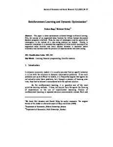
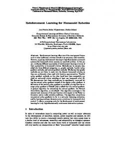
encounter, i.e. changes in delivery time lengths or changes in topology, the formerly found shortest path may loose its appropriateness. The need for good dynamic solution is required. A possible example can be seen in Figure 1, which is known as Internet Packet Routing problem.
In the paper RL-based implementation of the Internet protocol (IP) packet routing problem is considered. A network of adaptive and cooperative agents are to transport data following the shortest route in time from a source computer to a destination, even if the transfer capacities of connections change in time. In contrast to the famously used static routing algorithms, the proposed method is capable to cope with dynamic conditions as well. Other possible applications of RL are also treated in the paper, including The Travelling Salesman’s problem, which implies solving dynamic scheduling tasks as well. Keywords: reinforcement learning, dynamic optimization 1. BRIEF PROBLEM DESCRIPTION Finding shortest-path in respect to some optimality criterion while traversing a graph is not a novel problem. Several algorithms were developed, such as A*, simulated annealing or Dijkstra’s algorithm to solve this exercise (Ahuja et al, 1993). However most of these algorithms are mainly static, which means that when changes in the graph
Figure 1: The Internet Packet Routing problem’s chart In Figure 1 a network of computers (routers) can be seen belonging to a computer sub network. The objection of these routers is to transport data packages from the previously marked source, denoted by S, to the destination node D following the shortest possible route. The “shortest route” here refers to the shortest route in delivery time. Other criteria can also be considered, such as minimizing the number of hops, or delivery costs. The peculiarity of the problem here is that the bandwidth of routes among machines, or the topology may vary depending on several mostly unexpected factors. In some cases computers may even be down preventing them
from data delivery. The data transfer also shows some periodical daily and weekly changes. A reasonable routing algorithm must therefore take these variable circumstances into account.
where rt is the reward given in time step t, E(.) represents expected value, and h is the maximal time-horizon. This formula is usually defined for infinite horizon as ∞
E(
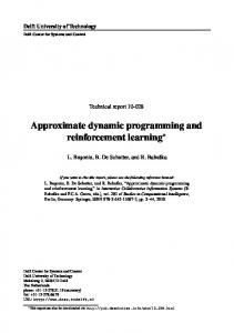
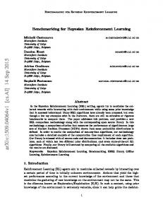
2. REINFORCEMENT LEARNING (RL) AS A POSSIBLE SOLUTION Reinforcement learning originates from dynamic programming (DP) and actor-critic algorithms (Nuttin, 1998). It is less exact than DP, since it uses experience to change system’s parameters and/or structure (Monostori and Viharos, 2000). DP uses iteration steps to update the model’s estimate of parameters about the real world: policy iteration and value iteration are tractable solutions in this case (Sutton and Barto, 1998). The schema of RL is shown in Figure 2.
Figure 2: Reinforcement learning in an agentenvironment interaction Here, a decision-making learning agent interacts with its environment. The agent can be described by states, out of a state set S. In each state, the agents choose an action, out of a set of available actions AS. Then the chosen action is evaluated by the environment, and a so-called reinforcement signal is supplied to the agent. This signal is a scalar value, high positive number for honored actions and huge negative number for dishonored actions. Such an agent, therefore, learns like a small baby trying to get as much good reward from its environment as possible in the long run. Partly due to the environment evaluation, or partly the state-change mechanism of the agent itself, the state may change asynchronously with the reward. In the special case of delayed reward the state may change several times, while waiting for the environment feedback. The goal of the agent is expressed as finding the maximal possible value of the following term: h
E(
∑
t=0
rt )
(1)
∑
γ t rt )
(2)
t=0
in discrete case, where γ ∈ [0,1] ⊂ R represents the discount factor, and ∞
E(
∫e
− βt
rt dt )
(3)
t=0
in continuous case. However, these expressions regard to the future expectation of rewards which is rarely known. These values can be estimated using recursive algorithms if, and only if, the transition probabilities between states or, more precisely state-action-next state triples are known, yielding a Markov decision process (MDP) (Nuttin, 1998). (Recursive equations solving MDP problems can be found in Appendix A.) However, in the case of an MDP this computation is computationally expensive facing to exponential-boom problems even for smaller graphs. A reasonable simplification in comparison with DP is to focus on the first action taken from the current state only, and suppose that the agent will behave optimally, i.e. choosing the best available action, thereafter. These considerations have led to the development of Q-learning (Sutton and Barto, 1998). 3. Q-LEARNING Q-learning considers only one state-action ahead, and defines Q-value for every state-action pair. This Q-value is proportional to the expected future reward of taking that action. Q represents an action-state value expressing how valuable is the selection of action a in state s for the system looking one step ahead only. The rule used to update Q values as advancing in time is as follows: Qt +1 ( s, a) = Qt ( s, a) + α (r + γ max Qt ( s' , a' ) − Qt ( s, a)) (4) a'
Here Q(s’,a’) denotes the action-state value of the next possible state, choosing optimal a’ (i.e. the next action), r the immediate reinforcement, and α is the learning rate of the agent. Having reached state s, action a must be chosen which maximizes, Q(s,a). This is referred to as greedy-method where in each state the best-rewarded action is chosen according to the stored Q-values. The term policy means assignment between states and actions. In each state, policy π is defined as π(s)=a, where action a yields the maximal reward during the next step in state s. However, in some cases actions which do not assure good immediate rewards should also be
chosen, because after a couple of decision steps the decision chain may provide much higher reward, than in the case of greedy steps. Therefore, the agent must carry out exploration when it selects an action. Exploration requirement reveals several possible methods for action selection. The three most popular action selection functions are greedy, ε-greedy and softmax action selection functions. Greedy-methods usually choose the best action, which in the case of Q-learning is the one with the highest possible action-state value. This method has the drawback of potentially running into local optima. In the case of ε-greedy methods agents choose best action a with probability of 1-ε, and select alternative actions randomly with the remaining ε probability ( ε ∈ [0,1] ). This function gives a certain chance to avoid local optima and find maximal long run reward. Softmax action selection makes action selection distribution dependent on a scalar temperature value T, which means that the agent chooses action according to the probability distribution, defined by Boltzmann’s formula. This formula also known from statistical mechanics is as follows: p (a i ) =
e Q ( s ,ai ) / T sk
∑e
,
(5)
Q ( s ,a j ) / T
j =1
where p(ai) is the selection probability of action ai, and sk is the number of selectable actions in state s and T is the temperature value. If T is relatively higher the differences in Q-values of variable actions are not emphasized, since the probabilities of selecting different actions are similar and, the probability distribution of the actions converges to unified distribution as T goes to infinity. Thus higher values of T encourages exploration of new actions (Sutton and Barto, 1998). If T is low enough the probability of selecting a poorly rewarded action is much smaller than selecting one with a high Q-value, which is usable in the exploitation phase. In this case the agent uses its knowledge greedily. T is often starts from higher values, and is decreased as the time advances. In some cases, especially, when some modifications occur in the environment the agent should bring-up its T value to enable further (or new) explorations. Cooling functions will be mentioned later in the paper.
addresses and next-hop computers. Internet Protocol addresses are used to uniquely identify each machine on the network. An example IP routing table of a UNIX workstation router process is inserted in Appendix B, and a relevant portion of an example CISCO router configuration file is put in Appendix C. So, going back to the fitting of RL and the IP Routing problem, the question is posed as: how could states, actions and rewards be formulated here? Actions are easy to identify as the addresses of next hops or, in the case of routers, the port numbers of outgoing communication lines. Each node connected to its neighbors only, so data packages can also be delivered only to them directly, but no other nodes. Therefore, an action is defined as delivering packets to a certain neighbor using a certain communication line. States can be identified at two levels. On the level of a network a state is defined as a source-destination tuple, so if a state changes it means modifications either in the source (data is transported from a different source), or the destination (data is sent to another destination). Both should mean to modify different rows in the table of Qvalues or Q-tables of different machines. Rewards are calculated as negative values of measured delivery times. Since delivery of packets is a process traversing different nodes along a path, a recursive Q-learning algorithm was wised to modify Q-tables of different routers, and learn through which nodes the shortest possible path can be approached. The schema of this algorithm can be found in Appendix D. The chosen action selection method uses Boltzmann’s formula, which enables exploration and exploitation balance using only one parameter, the temperature. Using higher temperatures, the selection probability of different actions are more or less equal. It is known from (Stefán, 2001) that if the Q-values are fixed integer numbers, an upper bound of the temperature values can be determined. Above this bound the exploration behavior is “good”, i.e. the unified distribution can be approached with a sufficiently small error. Following similar reasoning, a lower temperature bound can also be determined. Below this temperature the stochastic action selection policy can be considered greedy distribution1. Equations (6) and (7) express these temperature bounds. T max =
4. FITTING REINFORCEMENT LEARNING TO THE ROUTING PROBLEM In order to apply RL principles to Internet Packet Routing first the meaning of states, actions and rewards must be clarified. It would be a reasonable demand to fit the routing strategy to the current routing principles. Current routing algorithms usually maintain a routing table, which includes assignments between possible destination
Q max − Q min 1 ,1 + ε n } ln min{ 1 − nε
(6)
−δ
(7)
T min = ln
1
ε (1 − ε )( n − 1)
Greedy distribution means in this context a probability distribution in which selection of a certain action has probability of 1, while the others’ have probability 0.
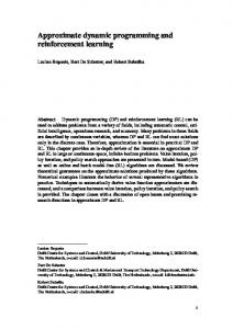
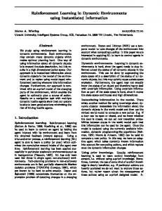
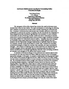
Here Tmax denotes the “exploration temperature”, Tmin the “exploitation temperature”, Qmax and Qmin the bounds on Qvalues; n is the number of actions available for a certain router (i.e. the number of its neighbors), ε is a small positive number representing the error of the approach, δ is the minimal difference between all possible Q-values. (Supposing that Qs are integers, the minimal value of δ is 1.) Tmax and Tmin mark off a temperature domain in which the balance between exploration and exploitation can be found. Theoretically, the minimal “exploitation temperature” is 0, but in practical applications, due to division by zero and floating point errors, a slightly higher value must be determined. If the number of time steps to carry out exploration is known, a cooling function between the temperature extremities can be defined based on the given time horizon. The two most commonly used approaches to handle the temperature in a multi-agent system are to apply: 1. a network-level temperature model or 2. an agent-level temperature model. The former means, that all nodes of the network share a common temperature value, thus the learning capability of the whole network can be controlled. In the latter case temperature values are assigned to each agent, which permits exploration in one part of the network, while the other part remain greedy. 5. IMPLEMENTATION IN JAVA Since testing of routing algorithms in real environment is a difficult and expensive exercise, a simulator has been developed in Java. Java holding object oriented principle proved to be a flexible and attractive tool for implementation. Furthermore a Java applet can run in a Web browser as well, so it is available to a great deal of potential testers on the net. The front page of the applet can be seen in Figure 3. In the figure, a single asterisk signs the source, and double asterisk does the destination node. Several parameters can be set on the control panel, such as: • learning rate (α), • discount rates (γ, η), • temperature (T) which the learning behavior of the whole network depend on. Currently, the network-level-temperature version of the software exist, i.e. the temperature of the whole network is the same. Before the implementation of agent-level temperature version, further investigation of the cooling behavior should be carried out. The chart of an example cooling function, and the delivery time vs. time steps are shown in Figure 4. Notice, that when the temperature is high (at about 200 degrees) the learning capability of the system is also high, thus high fluctuations in delivery time is observed. As the temperature decreases following stepfunction (solid, step-like curve in the picture), the system
become more and more greedy, thus, the system uses its knowledge, and the delivery time remains close to its minimum.
Figure 3: The graph in the Java simulator The crucial thing is how to decrease the temperature of the system in order to reach global near-optimal behavior. During the test run, the temperature was still adjusted by hand. The maximal and minimal temperature using equations (6) and (7) has been Tmax=2000 and Tmin=10. Other parameters were set as follows: α = 0.1 (learning rate) η = 1.0 (reward discount rate) ε = 0.1 (error of approaching extremities) γ = 0.9 (discount rate) The temperature was decreased from Tmax to Tmin according to a step-function, the step-value was set to approximately 200. A step decrease was taken at every 15 iteration steps. It was experienced that when the temperature was higher, delivery time fluctuated in a wide range, often taking graph cycles. When the temperature was lowered, the fluctuations became smaller and bellow a threshold T-value no deviations were experienced; the minimal distance was reached between the source and the destination. This optimal path was verified by Dijkstra’s static label-setting algorithm (Ahuja et al, 1996). Whenever changes in the graph encountered in terms of delivery time, raising the temperature up to Tmax again and bringing it to Tmin the
algorithm was able to discover a new shortest (or close-to shortest) path again in about 30 iteration steps.
A reinforcement learning model of job dispatching task in agent-based manufacturing environment will also be detailed in the near future. 7. ACKNOWLEDGEMENTS The authors would like to express their appreciation to András Márkus, József Váncza, Anikó Ekárt, Zsolt János Viharos, Botond Kádár and to Tibor Tóth for their conscientious and thorough help. REFERENCES
Figure 4:
Delivery time vs. time steps. An example cooling function is schematically put on the figure
6. CONCLUSIONS AND FUTURE WORK In this paper a model of adaptive shortest-path-finding algorithm have been introduced. Reinforcement learning has been proved to be a sufficient tool in creating cooperative, adaptive agents, which act in order to approach the global optimum. Tuning possibility of the learning capability of these agents using temperature bounds was also mentioned, and finally a basic version of an agent-based routing program written in Java was presented. Future investigations will be devoted to agent-level temperature formulation, testing the model with various learning parameters and to identify good cooling functions. We would also like to apply the model to special shortest path problems, such as the travelling salesman’s problem (TSP), in which case also the shortest path is to be determined, but with the constraints of visiting all nodes only once, and without any formal destination node2.
2
In the case of TSP the goal is to traverse the whole graph, so the destination is usually the source node itself having traversed all the nodes once.
Ahuja, R., Magnanti, T.L., Orlin, J.B. (1993), Network flows, Prentice Hall, ISBN 013617549-X Crites, R.H., Barto, A. (1995), An actor/critic algorithm that is equivalent to Q-learning, Advances in Neural Information Processing Systems, Vol. 7,MIT press Crites, P.H., Barto, A. (1996): Improving elevator performance using reinforcement learning, Advances in Neural Information Processing Systems, Vol. 8,MIT press Kaelbling L.P., Littman, M., Moore A.J. (1996): Reinforcement learning: a survey, Journal of Artificial Intelligence Research, Vol. 4, pp. 237-285 Monostori, L., Márkus, A., Van Brussel, H., Westkämper, E. (1996), Machine learning approaches to manufacturing, CIRP Annals, Vol. 45, No. 2, pp. 675712. Monostori, L., Kádár, B.; Viharos, Zs.J., Stefán, P. (2000), AI and machine learning techniques combined with simulation for designing and controlling manufacturing processes and systems, Preprints of the IFAC Symposium on Manufacturing, Modeling, Management and Supervision, MIM 2000, July 12-14, 2000, Patras, Greece, pp. 167-172 Monostori, L.; Viharos Zs. J.; Markos, S. (2000), Satisfying various requirements in different levels and stages of machining using one general ANN-based process model; Journal of Materials Processing Technology, Elsevier Science SA, Lausanne, pp. 228-235 Nuttin, M. (1998), Learning approaches to robotics and manufacturing: Contributions and experiments, Ph.D. Dissertation, PMA, KU Leuven. Ohkuara, K., Yoshikawa, T., Ueda, K. (2000), A reinforcement-learning approach to adaptive dispatching rule generation in complex manufacturing environments, Annals of The CIRP Vol. 49/1/2000, pp.:343-346 Stefán, P. (2001), On the relationship between learning capability and Boltzmann-formula, Technical Report, Computer and Automation Research Institute of the Hungarian Academy of Sciences Singh, S., Jaakkola, T., Littman, M., Szepesvári, Cs. (2000), Convergence results for single-step on-policy reinforcement-learning algorithms, Machine Learning, Kluwer Academic Publishers, pp. 287-308
Sutton, R., Barto, A. (1998), Reinforcement Learning (An Introduction) Tanenbaum, A. (1999), Computer networks, Panem Press, ISBN 963 545 213 6 Ueda, K., Hatono, I., Fujii, N., Vaario, J. (2000), Reinforcement learning approaches to biological manufacturing systems, Annals of the CIRP, Vol. 49/1/2000, pp. 343-346 Viharos, Zs. J. (1999), Application capabilities of a general, ANN based cutting model in different phases of manufacturing through automatic determination of its input-output configuration; Journal of Periodica Politechnica - Mechanical Engineering, Vol. 43, No. 2, pp. 189-196 APPENDIX A: VALUE ITERATION PROCESS Iterative equations solving Markov decision processes are about finding a quantity which measures how valuable is to be in a certain state s ∈ S in respect to the expected future rewards. This quantity is denoted by V and called value-function. Values for states can be determined by the formula as follows: ∞
V ( s ) = max ( E ( π
∑γ
t
rt )) , ∀ s ∈ S
(A1)
t=0
Here π represents the policy. When transition probability from state s to s’ via action a is known and is denoted by T(s,a,s’), (A1) becomes V ( s) = max( R( s, a ) + γ π
Destination ----------193.225.87.0 193.6.16.0 193.225.86.0 224.0.0.0 default 127.0.0.1
Gateway -------------193.225.86.254 193.225.86.254 193.225.86.254 193.225.86.254 193.225.86.15 127.0.0.1
Flag ---U U U U UG UH
Ref --5 5 5 5 0 0
I.face -----hme0 hme0 hme0 hme0 lo0
The first two columns are the most interesting, since destination here conforms the destination of the subnet or the destination machine; gateway is the next hop in the delivery chain. APPENDIX C: A CISCO routing table Configuration files of routers have also got adjacent routers’ notifications. A piece of a sample routing configuration file is included here: router bgp 1955 no synchronization network 195.111.0.4 mask 255.255.255.252 network 195.111.98.160 mask 255.255.255.240 neighbor 195.111.0.6 remote-as 3338 neighbor 195.111.0.6 description gw7 neighbor 195.111.0.6 route-map sztaki-in in neighbor 195.111.0.6 route-map sztaki-out out neighbor 195.111.97.1 remote-as 1955 neighbor 195.111.97.1 description gsr.vh.hbone.hu neighbor 195.111.97.1 update-source Loopback0 neighbor 195.111.97.1 route-map hbone-mag-out out no auto-summary!
APPENDIX D: Path-routing algorithm
∑ T (s, a, s' )V (s' )) ,
s '∈S
∀s ∈ S
Routing Table:
(A2)
where R(s,a) represents the given reward in state s choosing action a. This also means that the policy is chosen to a in state s which maximizes (A2) equation.
route(this_node,prev_node) return r { if destination is not reached then { choose action a at this_node out of the available set of nodes using softmax action selection method; determine next node next_node; ret:=funcmod(next_node,this_node);
APPENDIX B: The structure of a routing table
if prev_node is not source then { reinforce:=ret+weight(previous_node, this_node); } else { reinforce:=ret; } update Q(this_node,next_node) by r; return (Q(this_node,next_node),reinforce) } else if switched off machine is reached then { return (Q(this_node,next_node), high negative value) } else { return(Q=0,weight(previous_node,this_node)) }
Issue the command > netstat –nr
on UNIX systems. This command will give the routing table of an ordinary (non-router) machine.
}