Solving nonogram puzzles by reinforcement learning Frédéric Dandurand (
[email protected]) Department of Psychology, Université de Montréal, 90 ave. Vincent-d'Indy Montréal, QC H2V 2S9 Canada
Denis Cousineau (
[email protected]) École de psychologie, Pavillon Vanier, Université d'Ottawa 136 Jean Jacques Lussier, Ottawa, Ontario, K1N 6N5, Canada
Thomas R. Shultz (
[email protected]) Department of Psychology and School of Computer Science, McGill University, 1205 Penfield Avenue Montreal, QC H3A 1B1 Canada
empty cell. At the beginning, the state of all cells is unknown (often portrayed visually by a grey color), and the goal is to determine if each cell is empty (white) or filled (black), while satisfying all of the numerical constraints.
Abstract We study solvers of nonogram puzzles, which are good examples of constraint-satisfaction problems. Given an optimal solving module for solving a given line, we compare performance of three algorithmic solvers used to select the order in which to solve lines with a reinforcement-learningbased solver. The reinforcement-learning (RL) solver uses a measure of reduction of distance to goal as a reward. We compare two methods for storing qualities (Q values) of stateaction pairs, a lookup table and a connectionist function approximator. We find that RL solvers learn near-optimal solutions that also outperform a heuristic solver based on the explicit, general rules often given to nonogram players. Only RL solvers that use a connectionist function approximator generalize their knowledge to generate good solutions on about half of unseen problems; RL solvers based on lookup tables generalize to none of these untrained problems.
1 1 2 1 2
2 1
0
4
3
2 2 2 1 0
Figure 1 - Example of a 5x5 nonogram puzzle. In the initial state presented here, all cells are grey to indicate that the problem solver does not know yet if they should be filled (black) or empty (white).
Keywords: Nonograms; problem solving; reinforcement learning; distance-based reward; SDCC.
Nonogram puzzles Invented in Japan in the 1980s, nonograms (also called Hanjie, Paint by Numbers, or Griddlers) are logic puzzles in which problem solvers need to determine whether each cell of a rectangular array is empty or filled, given some constraints. Nonograms are interesting problems to study because they are good examples of constraint satisfaction problems (Russell & Norvig, 2003), which are ubiquitous in real life (Shultz, 2001). Furthermore, despite their popularity among puzzle players, little work on nonograms exists in cognitive science, either in the form of empirical studies or modeling work. But nonograms have attracted attention in other areas. For instance, as we will see in the literature review section, solving nonograms has been studied mathematically, and a number of machine solvers exist. Finally, many rules and strategies for human players are described in web sites. In nonograms, constraints take the form of series of numbers at the head of each line (row or column) indicating the size of blocks of contiguous filled cells found on that line. For example, in Figure 1, the first row contains 2 blocks of 2 filled cells, whereas row 5 contains no block of filled cells. Blocks have to be separated by at least one
Strategies for solving nonograms To solve nonograms, two important activities are necessary. First, the problem solver needs to decide which line (row or column) to solve next, and then to actually solve that line. Problem solvers typically need to iterate through the lines, progressively gathering more and more information about whether cells are empty or filled, until the actual state of every cell is known. Just as in crossword puzzles where the found words provide letters as clues or constraints for the orthogonally intersecting words, partially solving the cells on a nonogram line provides additional constraints for the intersecting lines. A survey of popular web sites giving advice and tips on how to solve nonogram puzzles was performed, focusing on categorizing advice on selection of a line to solve, or on how to solve a given line. The majority of the advice relates to solving lines. For instance, an exhaustive set of rules can be found on Wikipedia (January 10, 2012 version). In contrast, there is comparatively little advice on how to appropriately select the next line to solve, and much of this
1452
advice is given implicitly in commented solutions of specific problems. When available, explicit and generalpurpose advice for line selection can be summed up as follows: begin with lines for which the constraint is either 0 (in which case all cells on that line are empty) or equal to the length of the line (in which case, all cells are filled). Occasionally, advice is also given to the effect that, by adding the different constraints (including an empty cell between each block) one can look for those that fill up a complete line (e.g., the first row in Figure 1 with constraints 2 2 is completely known as XX_XX, with X as filled cells and _ as empty cells). Skilled players also realize that lines that contain blocks of large sizes are often a good place to start. Finally, another general piece of advice is to pay attention to lines that have changed due to updates of the cells of intersecting lines. Except for the last one, these general advice rules often consider block constraints only, and do not take into account additional constraints imposed by cells already known to be filled or empty. To sum up, strategies for solving lines are well-described as explicit, symbolic rules. In contrast, strategies for selecting lines appear more difficult to capture in explicit, symbolic terms, except for simple cases.
1 1 2 1 2
2 1
0
4
2 1 2
0
4
Nonograms have been studied mathematically, and are known to be NP-complete (Benton, Snow, & Wallach, 2006), making search-based solution techniques practical only for small problems. More sophisticated solving approaches include rule-based techniques (e.g., Yu, Lee, & Chen, 2011), use of some intersection mechanism to prune inconsistent configurations (e.g., Yen, Su, Chiu, & Chen, 2010), linear programming (Mingote & Azevedo, 2009), genetic algorithms (e.g., Batenburg & Kosters, 2004) and a combination of relaxations and 2-satisfiability approaches (Batenburg & Kosters, 2009). Nonograms also have been used as a tutorial for teaching university students about optimization using evolutionary or genetic algorithms (Tsai, Chou, & Fang, 2011). To our knowledge, there have been no attempts to use reinforcement learning to solve nonograms.
Our objective is to compare a solver for selecting the order in which to solve lines in nonograms based on reinforcement learning with three algorithmic methods: randomly, heuristically, and optimally (in the shortest number of steps). We thus ask if an RL-based solver can learn good solutions, that is, solutions that are close to the optimum (i.e., shortest solution); and how they generalize to unseen problems.
Figure 2 - Partial solution of a 5x5 nonogram puzzle.
2 1
Research on solving nonograms
Research objectives
3
2 2 2 1 0
1 1
eventually be determined. The final solution of the puzzle is given in Figure 3. In solving nonograms, the order in which lines are solved influences how many steps are necessary to complete the solution. A step is defined here as a single iteration on a specific line to extract the maximum information possible.
3
Methods
2 2 2 1 0
Generated nonogram puzzles Puzzles used for training and testing of the system have a size of 5 rows by 5 columns. The state of each cell (filled or empty) is randomly selected. The puzzle presented in Figure 1 was generated in this way, and used in the simulation. Only puzzles that have a unique solution are kept that is, puzzles for which block values correspond to one and only one board configuration. An example of non-unique problem is presented in Figure 4.
Figure 3 - Solution of the example 5x5 nonogram, where all cells are known to be filled (black) or empty (white) and where the solution satisfies all the block sizes constraints. Figure 2 presents an example of a partial solution of a nonogram puzzle after three steps. Column 3 and row 5 contain no block of filled cells, and thus all cells on them are empty. As described above, the first row is completely known. At this point, the position of the block of size 4 in column 4 is known, and so is the position of block 3 in column 5. Even though position of the blocks of size 1 in rows 2 and 4 cannot be determined yet, by propagating constraints from solving columns, their positions can
1 1 1
1
1
1
1 1
Figure 4 - Example of a non-unique puzzle. The right and the left configurations both satisfy the block size constraints.
1453
visited, after which a new round of visits is performed starting from the best remaining candidate lines. Similarly to the general advice and rules that can be found online, the heuristic solver does not take into account the current state of the problem.
Training and testing regimes RL solvers are incrementally trained on 3 different problems (starting with a single problem, and gradually increasing to three problems interleaved in the training set), and tested on a novel problem. A justification for these choices is presented in the Discussion section. Training proceeds on a single problem for 40 episodes, then training proceeds with problems 1 and 2 for 40 more episodes and finally the solver is trained on all three problems for 40 final episodes. Thus training involves 120 episodes in total. The reason for using this interleaved, incremental training (which rehearses problems already learned) is to avoid catastrophic interference (McCloskey & Cohen, 1989).
Optimal nonogram solver Here, a breadth-first search finds the minimal number steps. While this is feasible for the 5x5 puzzles considered here, experiments with larger puzzle sizes suggest that search time is prohibitively long -- a well-established result for NPcomplete problems, as mentioned1.
Optimal solver for lines Before discussing approaches to the selection problem, it is important to emphasize that simulations use an optimal line solver for solving a given line once it is selected. This optimal line solver can find all the new cells that can be declared as filled or empty. To find these cells, the optimal line solver module first generates every possible position of all blocks (constraints) in the line consistent with the cells already determined as filled or empty. Second, it computes the intersection of all these possible positions. Finally, it identifies cells that are always filled or always empty in these intersections as such cells are now known for sure to be filled or empty. This approach covers rules and strategies typically given to players for solving lines of nonograms, and implements rules described in other solvers (e.g., Yu et al., 2011). For instance, with a line that is currently blank (all unknowns), this method implements the rules described in Wikipedia (January 10, 2012 version) under "Simple Boxes" and "Simple spaces".
Modules for selecting lines to solve Given this optimal line solver for solving lines, we turn to the issue of selecting the next line (either a row or a column) to solve. Random solver A random solver randomly selects the next line to solve, with replacement, from lines that are not completely solved already. Selection with replacement allows taking the same line twice in a row. Heuristic solver A heuristic solver, inspired by the advice given to humans described above, selects order as follows. First, it chooses lines that have no block (easy case to solve because all cells are blank) and lines that are filled completely (e.g., 2 2). Then other lines are sorted and chosen in decreasing order of the largest block value. Lines with the same score (i.e., ties) are selected in the order in which they appear in the puzzle (rows then columns). Selection of the next line to solve is done without replacement until all lines have been
Reinforcement learning (RL) solver The reinforcement learning (RL) solver learns the expected value of lines using a reinforcement algorithm called SARSA (Sutton & Barto, 1998). SARSA learns estimates of the expected value or quality (Q) of future rewards for every state-action pair. Its learning rule is Q(st,at) Q(st,at) + α [ rt+1 + γ Q(st+1,at+1) - Q(st,at)] where Q is the predicted reward (sometimes called Quality), s is a state, a is an action, r is a reward, and indices t and t+1 are used for current and next states and actions respectively; α is the learning rate, and γ is the discount factor. The name SARSA is based on the quintuple that the algorithm uses (st, at, rt+1, st+1, at+1). In the present simulations, we use a learning rate of 0.9, and a discount factor of 0.9 to reward the shorter solutions more highly. States, actions and rewards are described below. States
For a given action (a choice of a line), the state given to the RL solver consists of the states of the cells on the corresponding line. In other words, the RL solver gets information that is directly relevant to the line considered, as the action will only affect the cells in the line considered. In human problem solvers, this corresponds to an attention mechanism that focuses on the relevant elements, rather than seeing the complete problem configuration. The state of a line consists of two elements: (1) the value of the block sizes coded using the integer corresponding to the number of cells in the block; and (2) states of cell on the line, which can take three values: unknown (U), filled (F) or empty (E), For example, in Figure 2, the state of column 1 is [1, 1, 0, F, U, U, U, E]. Note that learning begins in the initial state in which all cells of the board are Unknown, and that, for lines or columns composed of 5 cells, there cannot be more than three blocks
1 As an approximation, if each line had to be solved once and only once, there would be (n+n)! combinations of sequences, which quickly increases with n. For n = 5, we get 3.6 million combinations, for n = 6, we get 479 millions; and n = 7, we already have 8.7x10¹⁰ (In practice, lines often need to be visited multiple times; or in rare cases not need to be visited at all).
1454
Actions
An action is a choice of the next line to solve. As there are 5 rows and 5 columns, the maximal number of actions available is 10. As soon as a line is completely solved, it is not further included in the list of actions considered for selection. Given a list of actions and associated Q values, the RL solver needs to choose an action to execute. Action selection is performed with replacement (i.e., the same action can be taken again before all actions are visited). In testing mode, the solver uses a greedy technique called Hardmax which always selects the action with the largest Q value. In contrast, the solver uses a Softmax approach when in learning mode to allow exploration of the problem space. Under Softmax, every possible action can potentially be selected with a probability of selection increasing with the Q value. We limit the number of steps that are allowed for finding a solution to 25, a value that is large enough to find a solution by randomly selecting actions (see Random in Figure 5). When failing to solve within 25 episodes in testing mode, the RL solver is typically stuck repeatedly selecting an action which does not yield any progress. Rewards
To provide rewards for line selection, we use a variant of a distance-reduction heuristic called distance-based rewards (Dandurand, Shultz, & Rey, 2012). Here, we return a reward equal to the proportion of the currently unknown cells that are determined as filled or empty as a result of selecting this action (i.e., solving this line). For instance, if cell states of the line are [U F U U E] before performing the action and [U F F U E] after, then 1 of the 3 unknowns were discovered, and this action would be rewarded with 0.33.
The neural network used is called sibling-descendent cascade-correlation (SDCC: Baluja & Fahlman, 1994), a variant of cascade correlation (CC: Fahlman & Lebiere, 1990) with reduced network depth. CC has been successfully used to model learning and cognitive development in numerous tasks (Shultz, 2003). Whereas default SDCC parameters are optimized for pattern classification, more appropriate parameter values were selected here for function approximation, namely to allow for longer input and output phases (see details in: Dandurand et al., 2012). Input and output phases were allowed to last for 200 epochs with a patience of 50 epochs. Change threshold was set to 0.01 for input phases, and 0.002 for output phases. Finally, the score threshold parameter was set to 0.025, a value that is small enough to approximate the targets well while limiting overfit. A cache system is used to interface SARSA and SDCC because they have different processing requirements. More specifically, SARSA updates its approximation function Q after every action (called online learning). In contrast, learning in SDCC involves multiple patterns (input-output pairs) at once (called batch learning). SARSA updates the cache buffers until there are enough patterns to make a batch to train CC; details can be found in Rivest and Precup (2003).
Results First, we investigate the characteristics of the puzzles used for testing and training using the three algorithmic solvers. A sample of 20 simulations was run, with each simulation learning 3 different puzzles and different random initializations of neural networks. The numbers of steps necessary to solve these puzzles, plotted in Figure 5, suggest that puzzles are well-matched across training sessions and testing.
Storing Q values
Random
Heuristic
Optimal
25 Number of steps to solve puzzle
We compare two systems for storing the rewards associated with state-action pairs. The first one is a classical lookup table which, for each unique state-action pair encountered, stores the value of the reward. Values need to be initialized to a non-zero value (here, we used 0.05) so that probabilities of selection are non-null under Softmax. The second system consists of a connectionist function approximator. Instead of explicitly storing all Q values, a neural network is used to generate an approximation of the Q value as a single, real-valued output, taking the stateaction pair as input. The three possible cell states are coded using 2 bits: Filled (1 0), Empty (0 1) or Unknown (0 0). Thus, a line state is a 13x1 vector (3 block values + 5 cells * 2 bits per cell). Actions are coded as a 10x1 vector (5 rows then 5 columns) of binary values with the bit at the corresponding location set to 1, all others set to 0. Thus, for column 1 in Figure 2, the neural network function approximator receives as input the vector [1 1 0 1 0 0 0 0 0 0 0 0 1 0 0 0 0 0 1 0 0 0 0], corresponding to the concatenation of state and action.
20 15
10 5
0 Test
Train0
Train1
Train2
Figure 5 - Number of steps necessary to solve test and training nonogram puzzles using the three algorithmic solvers. Error bars represent standard errors (SE). Figure 6 shows performance results for the lookup table. As we can see, it learns near-optimal solutions for the training material (M = 8.5 and M = 7.6 for RL and optimal nonogram solvers respectively); outperforming the heuristic
1455
solver. However, RL solvers based on a lookup table do not generalize at all; performance on the test set reaching the maximal 25 steps on all 20 replications. 30
Number of steps to solve
25 Training set 1
Training set 2
20
Training set 3 15
Test set Random
10
Heuristic
Optimal 5
when good action is just below. We get back to this issue in the discussion. Finally, we compare the rewards learned by the SDCCbased RL solver with the scores given by the heuristic solver for the first move (i.e., step 1). We find a small but significant correlation of r = 0.18, p = 0.01, This suggests that RL solvers learned good solutions without needing to fully implement the advice often given to human players for solving the initial board condition. This is unsurprising, as the rules given to humans may not be optimal, and, with many steps necessary to solve these puzzles (at least about 9 steps), there are many possibilities to the optimization process beyond step 1.
Discussion
0
Figure 6 - Number of steps to solve nonogram puzzles with the RL solver using a lookup table, compared with the three algorithmic solvers, with standard error (SE) bars 30
Steps to solve
25 20
Connectionist function approximator Connectionist trials not at ceiling Lookup table
15
10 5
Random
Constraints on the choice of actions
Heuristic
Optimal
0
Figure 7 - Generalization performance (i.e. test set) of RL solvers using connectionist function approximators and lookup tables, with a ceiling at 25 steps, compared with the three algorithmic solvers, with standard error (SE) bars Next, we investigate generalization performance comparing the lookup table with the connectionist function approximator (see Figure 7). As we can see, the connectionist function approximator does generalize to good solutions of 9.1 steps (in the second column) for 7 of the 20 simulations. The other 13 are at ceiling, which, when included makes the average shown in the first column. Networks that reach the ceiling value typically get stuck selecting repeatedly an action that does not yield progress, due to the use of Hardmax and a selection strategy with replacement. Because Hardmax is only sensitive to the action with the largest Q value, the choice of action does not reflect learning all other actions2. In particular, Hardmax may select a poor action that obtains the best Q value, even 2
In general, performance differences between the heuristic and the RL solvers can be explained by the better choices that RL solvers make beyond the first solution step when the board is in its initial state. As mentioned, it is difficult to describe explicit and general purpose strategies for choosing lines to solve when the cells already solved place additional constraints. In fact, none of the online advice gives such explicit rules, but some advice implicitly provides guidance when describing solutions for specific problems. Similarly, RL solvers implicitly learn good choices for the next line to solve at any point in the solution, leading to near optimal solutions.
We have considered presenting results with Softmax, which does reflect learning of all actions. However, we found too much variability, and that performance was inflated due to capitalization on chance (randomly selecting good actions within the ten available).
As mentioned, by choosing the most flexible selection strategy, the one with replacement, networks need to learn their way out of repeatedly selecting the same action, leading to no further progress. In future research, different ways to handle this issue could be explored by placing additional constraints on action choice. For instance, RL solvers could keep track of the last N action choices made, and avoid selecting from these. With N = 0, we get the present "with replacement" scenario, whereas N = 10 (5 rows and 5 columns) would correspond to the "without replacement" scenario. Imposing this constraint would sidestep the need to learn their way out of repeated action choices.
Cognitive modeling To our knowledge, there are no experimental studies of humans solving nonogram puzzles. The present simulations make testable quantitative predictions about how humans choose which lines to solve, thus providing some guidance for such research As a cognitive model, the present system is hybrid, with a symbolic system for solving a given line, and a reinforcement learning with neural network support for choosing an appropriate ordering of lines. This modeling approach is grounded in evidence for both implicit and explicit cognitive processes (e.g., Reber, 1989). With Clarion (Sun, 2006) as a notable exception, modeling work on problem solving has mostly focused on explicit symbol
1456
manipulation. The present work addresses the implicit aspects of learning how to solve problems. The fact that advice and strategies found online have little to say about the order in which to select lines suggests that it may well be an implicit task, difficult to verbalize as explicit rules.
Towards a universal solver Our reinforcement learning (RL) solvers learn near-optimal ordering of lines to solve nonogram puzzles, outperforming a heuristic solver based on general purpose rules for line selection. Our solvers show that multiple problems (here, 3) can be learned by a single system, and that about half of them generalize to a novel problem when coupled with a function approximator to compute, rather than merely stores, expected rewards. These results are so far limited to puzzles of relatively small size. For future work, we could study generalization to larger puzzle sizes. Long term goals could include the design a universal solver that could solve any nonogram puzzle of various sizes nearly optimally. We tried training a RL solver with different, randomly generated nonograms on every learning episode, exploring some of the many simulation parameters (e.g., learning rates). These early attempts suggest that the task is difficult. In addition to the search space being very large, the function approximator appears to have difficulty learning stable representations when there is very high variability. Future research could also explore how to learn a larger number of problems (e.g., 10 or 100) in a reasonable time. Preliminary results suggest that it may be beneficial to gradually increase puzzle size.
Acknowledgments We thank Arnaud Rey for helpful comments on an earlier draft. This work is supported by a post-doctoral fellowship to FD and a grant to TRS, both from the Natural Sciences and Engineering Research Council of Canada.
References Baluja, S., & Fahlman, S. E. (1994). Reducing network depth in the cascade-correlation ( No. CMU-CS94-209). Pittsburgh: Carnegie Mellon University. Batenburg, K., & Kosters, W. (2004). A discrete tomography approach to Japanese puzzles. Proceedings of the 16th Belgium-Netherlands Conference on Artificial Intelligence (BNAIC) (pp. 243–250). Batenburg, K., & Kosters, W. (2009). Solving Nonograms by combining relaxations. Pattern Recognition, 42(8), 1672–1683. Benton, J., Snow, R., & Wallach, N. (2006). A combinatorial problem associated with nonograms. Linear algebra and its applications, 412(1), 30–38. Dandurand, F., Shultz, T. R., & Rey, A. (2012). Including cognitive biases and distance-based rewards in a connectionist model of complex problem solving. Neural Networks, 25, 41–56.
Fahlman, S. E., & Lebiere, C. (1990). The cascadecorrelation learning architecture. In D. S. Touretzky (Ed.), Advances in neural information processing systems 2 (pp. 524–532). Los Altos, CA: Morgan Kaufmann. McCloskey, M., & Cohen, N. J. (1989). Catastrophic interference in connectionist networks: The sequential learning problem. In G. H. Bower (Ed.), The psychology of learning and motivation (pp. 109–165). San Diego: Academic Press. Mingote, L., & Azevedo, F. (2009). Colored nonograms: an integer linear programming approach. Progress in Artificial Intelligence, 213–224. Reber, A. S. (1989). Implicit learning and tacit knowledge. Journal of experimental psychology: general, 118(3), 219–235. Rivest, F., & Precup, D. (2003). Combining TD-learning with Cascade-correlation networks. the Proceedings of the twentieth International Conference on Machine Learning (ICML) (pp. 632–639). Russell, S., & Norvig, P. (2003). Artificial intelligence, a modern approach. Second edition. Upper Saddle River, NJ: Prentice Hall. Shultz, T. R. (2001). Constraint satisfaction models. In J. Smelser & P. B. Baltes (Eds.), International Encyclopedia of the Social and Behavioral Sciences (pp. 2648–2651). Oxford: Pergamon. Shultz, T. R. (2003). Computational developmental psychology. Cambridge, MA: MIT Press. Sun, R. (2006). The CLARION cognitive architecture: Extending cognitive modeling to social simulation. In R. Sun (Ed.), Cognition and multi-agent interaction. New-York, NY: Cambridge University Press. Sutton, R. S., & Barto, A. G. (1998). Reinforcement learning: an introduction. Cambridge, MA: MIT Press. Tsai, J. T., Chou, P. Y., & Fang, J. C. (2011). Learning Intelligent Genetic Algorithms Using Japanese Nonograms. Education, IEEE Transactions on, (99), 1–1. Yen, S. J., Su, T. C., Chiu, S. Y., & Chen, J. C. (2010). Optimization of Nonogram’s Solver by Using an Efficient Algorithm. Technologies and Applications of Artificial Intelligence (TAAI), 2010 International Conference on (pp. 444–449). Yu, C. H., Lee, H. L., & Chen, L. H. (2011). An efficient algorithm for solving nonograms. Applied Intelligence, 35(1), 18–31.
1457