Atmos. Chem. Phys., 9, 5007–5025, 2009 www.atmos-chem-phys.net/9/5007/2009/ © Author(s) 2009. This work is distributed under the Creative Commons Attribution 3.0 License.
Atmospheric Chemistry and Physics
Reinterpreting aircraft measurements in anisotropic scaling turbulence S. Lovejoy1 , A. F. Tuck2 , D. Schertzer3,4 , and S. J. Hovde2 1 Physics,
McGill University, 3600 University st., Montreal, Que. H3A 2T8, Canada Earth System Research Laboratory, Chemical Sciences Division, 325 Broadway, Boulder CO 80305-3337, USA 3 CEREVE, Universit´ e Paris Est, France 4 M´ et´eo France, 1 Quai Branly, Paris 75005, France 2 NOAA
Received: 5 November 2008 – Published in Atmos. Chem. Phys. Discuss.: 4 February 2009 Revised: 14 May 2009 – Accepted: 30 June 2009 – Published: 27 July 2009
Abstract. Due to both systematic and turbulent induced vertical fluctuations, the interpretation of atmospheric aircraft measurements requires a theory of turbulence. Until now virtually all the relevant theories have been isotropic or “quasi isotropic” in the sense that their exponents are the same in all directions. However almost all the available data on the vertical structure shows that it is scaling but with exponents different from the horizontal: the turbulence is scaling but anisotropic. In this paper, we show how such turbulence can lead to spurious breaks in the scaling and to the spurious appearance of the vertical scaling exponent at large horizontal lags. We demonstrate this using 16 legs of Gulfstream 4 aircraft near the top of the troposphere following isobars each between 500 and 3200 km in length. First we show that over wide ranges of scale, the horizontal spectra of the aircraft altitude are nearly k −5/3 . In addition, we show that the altitude and pressure fluctuations along these fractal trajectories have a high degree of coherence with the measured wind (especially with its longitudinal component). There is also a strong phase relation between the altitude, pressure and wind fluctuations; for scales less than ≈40 km (on average) the wind fluctuations lead the pressure and altitude, whereas for larger scales, the pressure fluctuations leads the wind. At the same transition scale, there is a break in the wind spectrum which we argue is caused by the aircraft starting to accurately follow isobars at the larger scales. In comparison, the temperature and humidity have low coherencies and phases and there are no apparent scale breaks, reinforcing the hypothesis that it is the aircraft trajectory that is causally linked to the scale breaks in the wind measurements. Correspondence to: S. Lovejoy (
[email protected])
Using spectra and structure functions for the wind, we then estimate their exponents (β, H ) at small (5/3, 1/3) and large scales (2.4, 0.73). The latter being very close to those estimated by drop sondes (2.4, 0.75) in the vertical direction. In addition, for each leg we estimate the energy flux, the sphero-scale and the critical transition scale. The latter varies quite widely from scales of kilometers to greater than several hundred kilometers. The overall conclusion is that up to the critical scale, the aircraft follows a fractal trajectory which may increase the intermittency of the measurements, but doesn’t strongly affect the scaling exponents whereas for scales larger than the critical scale, the aircraft follows isobars whose exponents are different from those along isoheights (and equal to the vertical exponent perpendicular to the isoheights). We bolster this interpretation by considering the absolute slopes (|1z/1x|) of the aircraft as a function of lag 1x and of scale invariant lag 1x/1z1/Hz . We then revisit four earlier aircraft campaigns including GASP and MOZAIC showing that they all have nearly identical transitions and can thus be easily explained by the proposed combination of altitude/wind in an anisotropic but scaling turbulence. Finally, we argue that this reinterpretation in terms of wide range anisotropic scaling is compatible with atmospheric phenomenology including convection.
1
Introduction
Aircraft are commonly used for high resolution studies of the dynamic and thermodynamic atmospheric variables and they are indispensable for understanding the statistical structure of the atmosphere in the horizontal direction. However, aircraft cannot fly in perfect horizontal straight lines, indeed recently (Lovejoy et al., 2004), it was shown that NASA’s ER-2
Published by Copernicus Publications on behalf of the European Geosciences Union.
5008 stratospheric plane can have fractal trajectories. This means that the mean absolute slope increases at smaller and smaller scales being cut off only by the aircraft inertia. For the ER-2, the fractality of the trajectory could be traced to a combination of turbulence and the plane’s autopilot which kept the plane near a constant Mach number of 0.7, effectively enforcing long range correlations between the wind and the aircraft altitude. The interpretation of such data requires assumptions about the turbulence and the mainstream turbulence theories are virtually all isotropic – or at least “quasi isotropic”, i.e. with at most “trivial” (scale independent) anisotropies – whereas on the contrary the atmosphere apparently displays “scaling anisotropy”. To understand what this means, denote by 1v the fluctuation in a turbulent quantity v. “Horizontal scaling” means that over a horizontal lag 1x; 1v=ϕh 1x Hh whereas “vertical scaling” means that over a vertical lag 1z, 1v = ϕv 1zHv (ϕh , ϕv are turbulent fluxes, Hh , Hv are scaling exponents). Strict (statistical) isotropy implies ϕh =ϕv and Hh =Hv . However, if Hh =Hv but ϕh 6 =ϕv the system is only “quasi-isotropic” or “trivially anisotropic” (structures may be flattened in the vertical but the mean aspect ratio of vertical sections is independent of scale). “Scaling anisotropy” refers to the much stronger (scale by scale, differential) anisotropy which is a consequence of Hh 6 =Hv ; when Hh 1200 84 108 12.8 7.6 >400 30.4 384 40 100 260 52 64 3.6 48
1xc
seff
0.02 0.01 0.008 0.02 0.02 0.01 0.008 0.02 0.01 0.007 0.02 0.01 0.03 0.01
ε ×104 (m2 s−3 )
Shear ×106 (s−1 )
(m)
0.3 0.2 40. 0.2 0.4 0.2 0.3 1.2 30. 40. 0.4 0.4 0.2 0.5 5. 2.0
7.3 4.9 20.4 9.0 21.3 8.1 20.9 46.4 6.6 7.2 10.1 8.4 9.9 6.8 8.0 5.8
0.04
ls
0.14 0.05 0.07 0.03 0.08 0.09 0.25 0.10 0.13 0.60 0.09 0.11 0.05
slope (“pitch”) of about 0.12 m/km; this was typical for an entire leg. However, this overall estimate is obviously a very crude characterization; indeed in Lovejoy et al. (2004) it was Atmos. Chem. Phys., 9, 5007–5025, 2009
argued that the ER-2 stratospheric aircraft with special autopilot had a fractal trajectory: Sz (1x) = h|1z(1x)|i ≈ a1x Htr
(1)
where a is a constant, 1z (1x) is the altitude change over a horizontal lag 1x, “” indicates ensemble (statistical) averaging and Sz (1x) is the (first order) “structure function”. For the ER-2 it was found that Htr ≈0.55 with an inner (smoothing) scale of about 3 km (as a consequence of aircraft inertia smoothing of the otherwise large slope variations) and an outer scale of the fractal regime at about 300 km due to the slow rise (≈1m/km) of the aircraft due to its fuel consumption; the ER-2 roughly followed isomachs rather than isobars. The fractal dimension of the trajectory is Dtr =1+Htr ; for the ER-2, Dtr ≈1.55. In order to get a better idea of the typical slopes (s) as functions of scale, for each of the 16 short “legs” we estimated h|s(1x)|i=
h|1z|i =Sz (1x)/1x=a1x Hs ; Hs =Htr −1 1x
(2)
these are shown in Fig. 2. From the figure we see that the steepest mean slopes are at the smallest scales and vary from about 0.6 to 1.2 m/km. It appears that for lags (1x) greater than ≈3 km, the slopes follow a suggestive fractal 1x H s law with Hs =−2/3 which would result if the vertical displacement was proportional to the fluctuation in the horizontal wind speed, 1z∝1v and if the latter follow a Kolmolgorov law in the horizontal h|1v (1x)|i ≈ ε1/3 1x 1/3 (ε is the turbulent energy flux; we confirm this below). Since the lift and drag forces depend on the horizontal wind, a relation of the type 1z∝1v for perturbations is not implausible. If this explanation is correct, the deviations for 1x10, the spectra were averaged over 10 bins per order of magnitude in wavenumber. The spectra are compensated by dividing by k-5/3 so that the flat regions follow a Kolmogorov k-5/3 law corresponding to a Δx-2/3 law for the slope in fig. 2. The Kolmogorov law is found to hold well except at the lowest wavenumbers. The units of the wavenumbers are (km-1) the highest wavenumber corresponds to 2 samples, i.e. 2 s or 560 m.
of the 16 legs. For reference, we show in black the line s ≈ Δx corresponding Fig. 2for .eachThis shows the mean dimensionless slope (h|s(1x)|i, to Htr =1/3. The structure function S was estimated by averaging over all disjoint lags. Since the number of such decreases increasing Δx, the not soreference, good Eq. 2) as a function oflagsscale forwith each of the 16statistics legs.areFor for the large Δx; those for lags > Δxmax/2 are−2/3 based on essential a single atmospheric we show in black the line s≈1x corresponding to H structure and are not shown. The dashed horizontal line is the mean slope at the half tr =1/3. trajectory point (i.e. the mean over all trajectories of s(Δxmax/2) = 1.2X10⁻⁴). The structure function Sz was estimated by averaging over all disjoint lags. Since the number of such lags decreases with increasing 1x, the statistics are not so good for the large 1x; those for lags > 1xmax /2 are based on essentially a single atmospheric structure and are not shown. The dashed horizontal line is the mean slope at the half trajectory point (i.e. the mean over all trajectories of s(1xmax /2) = 1.2×10⁻⁴ ).
Fig. 3a. The horizontal spectrum of the altitude for each of the legs (1–16 bottom to top, each displaced by an order of magnitude for clarity). In order to see the trends more clearly, for k>10, the spectra were averaged over 10 bins per order of magnitude in wavenumber. The spectra are compensated by dividing by k −5/3 so that the flat regions follow a Kolmogorov k −5/3 law corresponding to a 1x −2/3 law for the slope in Fig. 2. The Kolmogorov law is found to hold well except at the lowest wavenumbers. The units of the wavenumbers are (km−1 ) the highest wavenumber corresponds to 2 samples, i.e. 2 s or 560 m.
be the result of aircraft inertia smoothing an otherwise even “rougher” trajectory. At large enough lags in Fig. 2 we see that each trajectory tends to a roughly constant mean absolute slope, although the lag and slope at which this occurs varies greatly from one trajectory to another from about 8 km to – in some cases – greater than the maximum i.e. >2000 km. These large 1x, “asymptotic” mean slopes – when they are attained – vary from about 0.3 m/km to ≈(40 km)−1 and a k −2.4 regime for k≈0 indicates that the altitude (pressure) fluctuations lag behind the wind fluctuations while θ −0.5
17
Fig. 3d: The first 4000 points (1120 km) of the legs (excluding number 7 which was too short) were used to estimate these ensemble spectra which were averaged over all the legs and over, ten wavenumber bins per order of magnitude (k in units of km-1). The pressure (red, top) and altitude (green, second from top), the transverse (orange, bottom) and longitudinal (green, bottom) winds are shown with reference lines indicating the theoretical vertical spectrum (k-2.4) and the theoretical horizontal spectrum k-5/3. The average transition wavenumber is about (30 km)-1.
-2
iii) k (40 km)−1 the vertical fluctuations are not dominant and the spectrum is the (apparently unbiased) horizontal Kolmolgorov value 5/3 where as for k1xc , while for small scales 1x