Relative Distance Based Localization for Mobile Sensor Networks

Relative Distance Based Localization for Mobile Sensor Networks Ji Luo and Qian Zhang Hong Kong University of Science and Technology {[email protected], [email protected]} Abstract—Many sensor network applications exploit the mobility angles. It is dramatically accurate but not cost efficient. of sensor nodes and the location-awareness plays an important 2. Range-free approaches. With range-free localization role in these applications. However, it is too expensive to equip algorithms, no special hardware is required to detect the special hardware in each sensor node for localization, thus a exact point-to-point distance or delivery angle. Most distributed range-free localization scheme in mobile sensor range-free algorithms require the location knowledge of network is highly desired. Several such localization techniques some beacon sensors as seeds before estimating position have been developed but few of them consider leveraging the of others. It maybe less accurate than range-based ones. feature of node mobility. Leveraging node mobility, in this paper, However the corresponding estimation errors can often be both static constrain set by transmission range and velocity masked through fault tolerance, redundancy etc. constrain set by node movement are introduced. Based on these In this paper, we target at a range-free localization scheme in two types of constrain, we propose a range-free Mobile Inequality mobile sensor networks: most nodes with unknown locations Localization (MIL) algorithm, which uses ring inequalities to and few seeds know their locations. We work on a very general restrict and estimate the possible location in numerical method. scenario, in which both the nodes and seeds are moving. There Our approach is distributed, quickly re-localizable and works are several challenges for utilizing range-free based solution: well when all sensors are moving uncontrollably. We analyze the 1) centralized algorithms can not work well as the node theoretical bound for the accuracy of the position estimation and mobility makes the routing protocol difficult to gather all the the comprehensive simulations demonstrate that our algorithm needed information; 2) quick re-localization is essential since performs much better than the existing works. the position of sensor are varying all the time; 3) information Keywords—Localization, mobile inequality localization, mobile which comes by multi-hop estimation maybe outdated because sensor networks, relative distance, range-free, ring inequalities. the position may has already changed. Thus a distributed and quickly re-localizable range-free algorithm is highly desired. I. INTRODUCTION Deployment of low cost wireless sensors is proving to be a It can be seen that all the above mentioned challenges are promising technique for many applications. Recently, mobile related to the node mobility. Though mobility brings new sensor networks are widely used since many applications such challenges, we can exploit it to improve the accuracy of node as seabed monitoring, animal tracking, river flow discovering localization. We have two observations which can form two and mapping depend on the mobility of sensor nodes. types of constraints on location in the mobile sensor network: Localization is one of the most important technologies since one is the relative distance constraint between sensors and the most applications such as ZebraNet [1], CarTel project [2] other is the relative distance constraint between positions of one sensor at different time. The first one depends on the depend on the location awareness. Localization is the ability of a sensor to find out its physical transmission/communication range. The latter one depends on coordinates. A straightforward approach would use GPS to the velocity of a sensor. A nice feature is that these two above obtain the absolute position of node. However, GPS-based observations can be achieved by distributed way in short systems require expensive and energy consuming electronics period of time. The essential idea about our work is then to for precise synchronization with the satellite’s clock. From the utilize the observations to develop enough relative distance viewpoint of deploying this technology in a large-scale sensor constraints for accurately estimating the position of sensor. network, one can only selectively deploy GPS in very few The paper makes four major contributions to the localization nodes of mobile sensor networks. Many localization problems in such a general framework. algorithms have been proposed to estimate per-node location 1. Range-free with low seed density. Our algorithm requires no information for sensor network. With regard to the special hardware except some beacon seeds. It can works in a mechanisms used for localization, there are mainly two types very low seed density which is really cost effective. 2. Leverage feature of mobility. The scheme proposed in this of approaches: range-based and range-free. 1. Range-based approaches. In range-based techniques, paper addresses the localization issue by exploiting mobility to sensors use special hardware to estimate some useful constrain sensor’s position. This actually creates a new angel information such as Time Difference of Arrival (TDoA), to consider the issues related to mobile sensor. Angle of Arrival (AoA) and Received Signal Strength 3. Effective Localization. Much better performance can be Indicator (RSSI) to get the information of distances or obtained compared with the traditional “bound box” scheme. 4. High accuracy in simulation. The comprehensive simulation demonstrated a high accuracy. We compared our results to This research was supported in part by the National Basic Research other algorithm such as Centroid [9], MCL [10]. Program of China (973 Program) under Grant No. 2006CB303100, the The rest of the paper is organized as follows. We will provide Key Project of Guangzhou Municipal Government Guangdong/Hong Kong Critical Technology grant 2006Z1-D6131, and the HKUST background and related works in Section II and introduce our Nansha Research Fund NRC06/07.EG01.

1076 1930-529X/07/$25.00 © 2007 IEEE This full text paper was peer reviewed at the direction of IEEE Communications Society subject matter experts for publication in the IEEE GLOBECOM 2007 proceedings.

algorithm in Section III and the corresponding protocol in Section IV. A simulation report will be given in Section V.

III. OUR SOLUTION: RELATIVE DISTANCE CONSTRAINT BASED LOCALIZATION

II. BACKGROUND AND RELATED WORK In wireless network, a great number of research works have been conducted for localization. Some general surveys can be found in [6] [7]. We will provide a brief survey of them and point out the differences with our work. Doherty [8] pioneered a typical centralized algorithm: the semi-definite programming (SDP) approach. All the constraints in semi-definite programming are expressed as linear matrix inequalities (LMIs). However, not all geometric constraints can be represented as LMIs. Without relaxing constraints, Camillo Gentile [3] developed an approach to transforming most of them into linear triangle inequalities and ensures a tighter solution. In our work, we propose ring inequalities to represented the constraints and solve them in distributed way. Many range-based techniques are developed based on using special hardware to estimate TDOA [9][10], AOA [11] and RSSI [12][13]. Recently, some interesting approaches were designed to achieve the same information without special hardware by adjusting the transmission range. W.-H. Liao and Y.-C. Lee [14] designed a method to change the transmission power levels to know the distance between nodes and beacons. However, adjusting the transmission range is not suitable for the scenario that all sensors are moving around in the network. Centroid [4] provides a simple idea of distributed range-free localization. Each node estimates its position using the center of the positions of all seeds which are its neighbors. However, in our scenario, the seeds are moving all the time. We can not explicitly deploy seeds to certain concrete position. All the work above hasn’t considered using the mobile sensor. N. B. Priyantha [15] proposed a new approach named MAL (Mobile-Assisted Localization) by using the mobile sensor to assist in localization. MAL employs mobile sensors to help measuring distances between nodes until these distance constraints form a “globally rigid” structure that guarantees a unique localization. Two biggest differences from our work here are 1) we can not control them moving as we want; 2) we want to develop a range-free based solution. The first piece of work that targets at the similar scenario as our work in mobile sensor network is pioneered by L. Hu and D. Evans [5]. They proposed an approach, MCL, which applies the Sequential Monte Carlo method to achieve localization. MCL is range-free and works when the motion of nodes is uncontrollable. MCL represents the posterior distribution of possible positions using a set of weighted samples. It uses Monte Carlo method to do the sampling and estimate the position. Our work provides a different geometrical way. We focus on the relative distance constraints, making use of mobile seeds to bring more constraints and using ring inequalities to represent them. After that, we solve those inequalities for estimating the position by a numerical method. MCL does not work well when the velocity is low and the samples are hard to collect in random way. Moreover, our work proves the theoretical bound of the estimate error in probability and the computational complexity for each node.

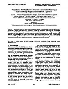
A. Motivation In wireless networks, node can know whether another node is in its transmission range by broadcasting a message to its onehop neighbors and check the feedback. If one node is in the transmission range R of another node, the distance between them won’t exceed R. This can naturally offer static constraint obtained from transmission range. Fig. 1 shows a simple example of these relative distance constraints for a node A.

Figure 1. Basic illustration for relative distance constraints

The mobility provides a special feature of mobile sensor network: velocity constraint. For example, assume every node can move within a maximum distance V at one time slot. If we have a relative distance constraint that the distance between two nodes is smaller than R, then after one time slot, the distance between these two nodes is smaller than R+2Vmax as shown in Fig. 1. With these two types of relative distance constraints, the possible position of node A can be restricted in certain area (e.g. the gray area in Fig. 1). More accurate estimation can be obtained when the sensor node obtains more and more constraints from the neighboring nodes broadcasting and its own movements. The basic idea of our proposed scheme then is composed of two phases: the first phase is to get many relative distance constraints using information from “transmission range” and “velocity” for every node and the second phase is to conduct the accurate location estimation on each node based on these constraints. B. Relative Distance Constraint generation Without losing the generality, we assume time is divided into discrete time slots. It is necessary to do re-localization in each time slot since nodes are moving uncontrollably. There’re mainly two types of constraints, one is the static constraint derived from transmission range and the other is the velocity constraint derived from the node mobility. 1) Static Constraint

Figure 2. Constraints of k-step neighbors

Let the transmission range be a constant R, at every time slot we have basic relative distance constraints: if one node is in the transmission range of another, the distance between them is no greater than R. These two nodes are called “1-step neighbors”. Furthermore, we can have “2-steps neighbors” that also gives the relative distance constraint that the distance between these


two nodes are greater than R but won’t exceed 2R. Fig. 2(a) and Fig. 2(b) show the example of 1-step and 2-step neighbors. We can extend these constraints to “k-steps neighbors” (k >2). However, the constraints of k-steps neighbors will be less powerful while k increases and the information collection come from multi-hops will delay the re-localization. Therefore, we only consider 1-step and 2-steps neighbors in our work. 2) Velocity Constraint It is a new type of constraints that is unique for mobile sensor which considers the distance between positions of one node in two consecutive time slots won’t exceed Vmax. Based on this feature and the neighboring relationship at different time slot, we have new constraints called “Motion on Boundary”. More specifically, if node A and B are not “1-step neighbors” in a previous time slot, then at current time slot the distance between them will be greater than R-2Vmax and smaller than R. That means B is just moving on the edge of A’s range. Furthermore, this velocity constraint can be applied on any existing constraints. Generally, if we have an inequality a ≤ ( x − c ) 2 + ( y − d ) 2 ≤ b to represent a relative distance constraint at previous time slot, then we will have the relative distance constraint in current time slot as shown in Eq. (1). This type of constraints is named as “Inherited Constraint”. (max of {0, a − Vmax })2 ≤ ( x − c) 2 + ( y − d ) 2 ≤

(

b + Vmax

)

2

(1)

In summary, we have “1-step neighbors” and “2-step neighbors” from transmission range and “Motion on Boundary” and “Inherited Constraint” from the mobility of nodes. All these constraints can be represented by ring inequality pattern: a ≤ ( x − c ) 2 + ( y − d ) 2 ≤ b . C. Position Estimation The relative distance constraint is between two sensors. If the position of one node is known (such as beacon) then the location of the other node is restrict in a ring area by one inequality. A node may have many relative distance constraints with other nodes and its location should be in the common area of all those ring areas. We call the common area as solution area whose shape maybe very complex as shown in Fig. 3.

while P increases the more simple shapes we have the higher accuracy of center we will get and the tradeoff is the cost of computing increases.

Figure 4. “Weighted center” based position estimation

IV. PROTOCOL DESIGN We name our protocol MIL (Mobile-Inequality Localization). In our work only the relative constraints which are between node and seed will be utilized. For every node, the protocol will store the observations and constraints as a neighbor-list and constraint table (store constraint inequalities). The protocol will re-collect the observations and update the neighbor-lists and constraint tables at each time slot. A. Collection and Update A seed says a hello message with its position in its transmission range. The node which receives the hello message will update the neighbor-list. Every node also broadcasts a message of its neighbor-list in its transmission range. A node receives these neighbor-lists will update its “neighbors’ neighbor-list”. Basing on the update of neighbor-list and “neighbors’ neighbor-list”, the constraint table will be updated. Moreover, if a seed is not in the neighbor-list of a node at previous time slot, but at current time slot, the seed comes into the neighbor-list. We can easily know which seeds are “Motion on Boundary” and update the constraint table. For every inequality a ≤ ( x − c ) 2 + ( y − d ) 2 ≤ b in constraint table at previous time slot, a new inequality (max of {0, a − Vmax }) 2 ≤ ( x − c) 2 + ( y − d ) 2 ≤

(

b + Vmax

added in current constraint table. Table 1.

)

2

will be

The construction of a Constraint Table

Figure 3. Simple illustration for “bound box” idea

One idea is to use a simple shape such as “Bound Box” [16] which is similar to the solution area but easy to represent and calculate its center alternative to the center of solution area. To achieve high accuracy, we use the combination of many simple shapes to represent a solution area. The essential idea is to calculate the center of each simple shape individually and then combine them into the average weighted center by using the area of each simple shape as weight. This average weighted center is used to approximate the estimate position of the node. We divide the “Bound Box” into P columns (column 0, 1,…, P-1) by X axis. For every column k, calculate the segments of solution area as shown in Fig. 4. The combinations of inner segments will be more similar to the original solution area than the outer bound box. As we divide the area into many columns,

Table 1 gives a chart to conclude the construction of a constraint table for a node. In the figure, we can see that a part of current constraint table, the “Inherited Constraint”, is generated by the previous constraint table. The size of constraint table grows as time goes on that means the storage requirement of a sensor increases. To control the size of constraint table, we adopt a cyclic array to keep the K newest inequalities. We will show the relationship between K and accuracy in the simulation of Section VI. After update the constraint tables, the protocol can start to calculate and


estimate the position of the node. B. Position Estimation The constraint table contains a number of inequalities, a ≤ ( x − c ) 2 + ( y − d ) 2 ≤ b . The position (x, y) of node should satisfy all inequalities. We use a numerical method to estimate the position by dividing the solution area into P columns. For a particular column i, there maybe more than one rectangular shapes (or segments) in the solution area. It has several steps to compute the possible segments in solution area: 1. x is fixed as X (i ) = X min + ( X max − X min ) × ( 2i + 1) /(2 P ) 2. For every inequality (ai , bi , ci , d i ) in constraint table, calculate the end-points of Y-axis as d i ± a i − ( x − ci ) 2 and d i ± bi − ( x − ci ) 2 .

3. Sort these end-points in ascending order so that every two adjacent end-points form a segment. We select those segments whose mid-points satisfy all inequalities in the constraint table L U and let [Yij , Yij ] to represent these segments of column in solution area. After achieving the possible segments of every column, we can compute a “Weighted Center” to estimate the position of node as shown in Eq. (2): X = ∑ ∑ X (i )(YijU − YijL ) ∑ ∑ YijU − YijL i

j

(

)

(

i

Y = ∑ ∑ (YijU + YijL )(YijU − YijL ) i

j

j

(

)

) 2∑ ∑ (Y

U ij

i

− YijL

j

)

(2)

In summary, the MIL protocol uses broadcasting messages in one hop to build neighbor-lists and constraint tables based on previous neighbor-lists and constraint tables. It supports two methods to estimate the position of nodes: one is center of “Bound Box” and the other is “Weighted Center”. We will analysis the theoretical accuracy, the overhead and the computation and space complexity in Section V. Then the comprehensive experiment will be conducted to compare the accuracy between two estimation methods in Section VI. V. PERFORMANCE ANALYSIS A. Theoretical Bound Estimate error is one of the most important metrics in evaluating the performance of a localization algorithm. We define the estimate error as the ratio of Euclidean distance between estimate-position and real-position and the transmission range R. At certain time slot, let the real-position of a node be (Xr, Yr) and the estimate-position be (Xc, Yc), the estimate error δ is defined in Eq. (3): δ=

( X r − X c ) 2 + (Yr − Yc ) 2

We have proved a lower bound of the probability of estimate error δ that is no greater than a value ε .

(

)

2

Sd   = 1 − (1 − ε ) π  , ε ≤ 1 ( 4)   Due to the space limitation, we will not include all the derivation details in this paper. It shows an important conclusion that: high seed density leads less error. The lower bound is achieved by only considering the constraint

P(δ ≤ ε ) ≥ 1 − (1 − ε )

m 2

VI. PERFORMANCE EVALUATION In this section, we do the simulation of MIL protocol by evaluating the estimated errors in various network and algorithm parameters. We will also compare our simulation results to other localization algorithm such as Centroid [9] and MCL [10] in the same environment. Our experiments are done by a special designed simulator which implements Centroid, MCL and our algorithm together. A. Simulation Environment Sensor nodes are randomly deployed in a 300m x 300m rectangular region. We assume the transmission range R is fixed by 30m for both nodes and seeds. We define the speed as the moving distance of one sensor per time slot. It can be divided into two types: node’s speed and seed’s speed. A node’s speed is randomly chosen from [Vmin, Vmax] and a seed’s speed is in the range of [Smin, Smax]. We use the classical random walk model in the simulation. B. Accuracy and Convergence Time

(3)

R

2

of 1-step neighbor and 2-step neighbor. In section VI, we will show that after using all constraints, the estimate error will be much smaller than we have in the analysis of theoretical way. B. Overhead We measure the communication overhead as the size of messages a sensor needs to send in localization process. In our localization protocol, the broadcasting operation will be executed by seeds and nodes at every time slot. For seeds, they will broadcast a hello message containing a name, position and some recognize-bits which is totally only several bytes. For nodes, they will broadcast their neighbor-list and neighbor’s neighbor-list in one hop. According to low seed density, it is about hundred of bytes. C. Computational Complexity Every node will do computation to estimate its position at every time slot. We divide the solution area into P columns. For each column there maybe 4K end-points of Y axis which should be sort to form segments, in about O(KlogK) time. For each segment, we will test whether it satisfies all K inequalities in the constraint table. Thus the total complexity is about O(P(KlogK+K2))=O(PK2). In our experiments, P=50 and K=50 is adequate for rather precise localization, so the computational complexity of each node is endurable for sensor nodes.

Figure 5. Accuracy Comparisons. (Sd = 2, Nd = 10, Vmax = Smax = 0.2R)

The estimate error of MIL depends on the number of sufficient inequalities. As time goes on, nodes will receive more information (constraints) and improve their estimate location errors. However, the error will converge finally since the number of stored constraints won’t increase any more after there are K inequalities in constraint table for each node. Thus, the variation of estimate errors can be divided into two phases:


one is the startup phase and the other is the stable phase. Fig. 5 compares Centroid, MCL and MIL. MIL has four types of constraints which can build the constraint table quickly and it use sufficient inequalities to depicture the possible location area strictly while MCL only does random sampling so MIL performs better in general. C. Moving Speed Different maximum speeds illustrate different features of mobility. Centroid does not consider the history information so the variation of maximum speed won’t affect the accuracy of stable phase. Since faster moving nodes will encounter more seeds and rapidly filter inaccurate samples in MCL so the estimate error decreases as maximum velocity increases. The estimate error of MIL also depends on the speed. We leverage the mobility to achieve constraints such as “Motion on Boundary” which restricts the distance in the range of [ R − 2Vmax , R ] . Higher speed will make the constraints less powerful so the estimate error may increase.

important issue. With limitation of sensor capability, we target at range-free solution for the scenario that both sensor nodes and seeds move uncontrollably within a maximum velocity. The core observation of our work is relative distance constraint that can be obtained from transmission range in both static network setup and movement velocity of the mobile sensor nodes. Our solution leverages the mobility to potentially improve the estimation accuracy. A more accurate position estimation method, “weighted center”, is introduced after obtaining enough independent constraints. The paper proposes a distributed protocol, MIL, for localization in a general network. It requires low seed density, very small overhead and computational complexity. The estimate error is really low and can fit most location awareness requirements. The algorithm also broadens the idea that using the ring inequalities to represent the location constraints and solving them by numerical method. It can be extended to range-based algorithm that the real distance between sensors should be in the range of [ d − ε , d + ε ] where d is the estimate distance and ε is the maximum error. We can apply an inequality to express this information in range-based algorithm. Future work will also focus on the security to avoid the impact of fake information in mobile sensor network. REFERENCES [1]

Figure 6. Comparisons with different speeds (Sd = 2, Nd = 10)

Fig. 6 shows a general view of estimate error in different maximum speeds. It is seen that the accuracy of Centroid does not vary too much while the estimate error of MCL decreases quickly as we desired. MIL begins to degenerate to MCL while maximum speed is around 0.5R. It is called “degenerate speed” since at this speed the range [ R − 2Vmax , R] provided by “Motion on Boundary” is [0, R] which degenerates to the constraint of “1-step Neighbors” and “Motion on Boundary” won’t provide any useful constraints above this speed. D. Seed Density

[2] [3] [4] [5] [6]

[7] [8] [9] [10] [11] Figure 7. Impact of seed density. (Nd = 10,Vmax = Smax = 0.2R)

As shown in Section V, the more seeds we have the more constraints a node may have. Increasing the density of seeds will make the estimate error smaller but the cost of the network and deployment will also increases. Fig. 7 shows the average estimate error in mobile sensor network with different seed density. MIL improves MCL in about 35% and can achieve an adequate accuracy when seed density is low. VII. CONCLUSION Localization for mobile sensor networks is a challenging and

[12] [13] [14] [15] [16]

The ZebraNet Wildlife Tracker, http://www.princeton.edu/~mrm/zebranet.html, Princeton University. B. Hull, V. Bychkovsky, K. Chen, M. Goraczko, A. Miu, E. Shih, Y. Zhang, H. Balakrishnan, and S. Madden, “CarTel: A Distributed Mobile Sensor Computing System”, SenSys 2006. C. Gentile, “Sensor Location through Linear Programming with Triangle Inequality Constraints”, Communications, 2005. ICC 2005. 2005 IEEE International Conference on Volume 5, 16-20 May 2005 N. Bulusu, J. Heidemann, and D. Estrin, “GPS-less Low Cost Outdoor Localization For Very Small Devices”, IEEE Personal Communications Magazine 2000. L. Hu and D. Evans, “Localization for mobile Sensor Networks”, MobiCom 2004 K. Langendoen and N. Reijers, “Distributed localization in wireless sensor networks: a quantitative comparison”, Computer Networks: The International Journal of Computer and Telecommunications Networking archive Volume 43 , Issue 4 , Nov. 2003. V. Chandrasekhar, W. KG Seah, Y. S. Choo and H. V. Ee, “Localization in underwater sensor networks: survey and challenges”, WUWNet’06, September 25, 2006. L. Doherty, K. S. J. Pister and L. El Ghaoui, “Convex Position Estimation in Wireless Sensor Networks”, IEEE InfoCom 2001 A. Savvides, C. Han, M. B. Strivastava, “Dynamic fine-grained localization in Ad-Hoc networks of sensors”, MobiCom 2001. N. B. Priyantha, A. Chakraborty and H. Balakrishnan, “The Cricket Location-Support System”, MobiCom 2000. D. Niculescu and B.i Nath. “Ad Hoc Positioning System (APS) Using AoA”. IEEE InfoCom 2003. P. Bahl and V. N. Padmanabhan, “RADAR: An In-Building RF-Based User Location and Tracking System”, IEEE InfoCom 2000. J. Hightower, G. Boriello and R. Want, “SpotON: An indoor 3D Location Sensing Technology Based on RF Signal Strength”, University of Washington CSE Report #2000-02-02, February 2000. W.-H. Liao and Y.-C. Lee, "Localization with Power Control in Wireless Sensor Networks", ICSNC 2006 N. B. Priyantha, H. Balakrishnan, Erik D. Demaine and Seth Teller, “Mobile-Assisted Localization in Wireless Sensor Networks”, IEEE InfoCom 2005. S. Simic and S. Sastry, “Distributed Localization in Wireless Ad Hoc Networks”, UC Berkeley Technical Report No. UCB/ERL M02/26.
