the data originates and ends at terminal nodes only, and we need disjoint paths between the terminal nodes. We call these additional nodes relay nodes. Relays ...
Relay Placement and Movement Control for Realization of Fault-Tolerant Ad Hoc Networks* Abhishek Kashyap and Mark Shayman Department of Electrical and Computer Engineering, University of Maryland, College Park MD 20742 Email: {kashyap, shayman}@eng.umd.edu
Abstract— Wireless communication is a critical component of battlefield networks. Nodes in a battlefield network exist in hostile environments and thus fault-tolerance against node and link failures is a desirable property for the communication topology of such networks. The network nodes are mobile and move depending on the objective they try to achieve; thus the topology needs to be re-established periodically. The transmitters used for communication have a fixed transmission range, so additional nodes are required for the construction of a fault-tolerant topology among network nodes. As the network nodes move, the additional nodes need to be moved as well; and it is desirable to move them a minimum amount to re-establish the topology as quickly as possible. We propose algorithms for minimizing the number of additional nodes required and the distance they need to move for construction of a topology with desired levels of fault-tolerance. We show via extensive simulations that the algorithms perform much better than an algorithm that does not take minimizing the movement of additional nodes into account.
I. I NTRODUCTION Battlefield communication networks are networks of mobile nodes, communicating with each other using wireless links. The nodes in the battlefield refer to soldiers, army vehicles, UAVs, robots, etc. The network may also be a team of nodes engaged together to perform a large scale reconnaissance mission. The capability of a device to communicate with all nodes (using single or multiple hops) is very critical for the collaborative missions to succeed. In these applications, the nodes are in hostile conditions, and the nodes or communication links between nodes may fail. Thus, it is critical for the communication network between the nodes to be connected even after a few failures. Also, since the nodes are mobile, it is necessary to re-configure the communication topology as it changes substantially. We model the communication topology as a graph on the nodes, assuming a fixed transmission range for each device. Each device is considered to be a vertex in the graph, and an edge exists between two vertices if they are within each other’s transmission range. Fault-tolerance is tolerance against device and link failures, thus we refer to fault-tolerance as the existence of k (> 1) edge-disjoint (or k internally vertexdisjoint) paths between each pair of vertices in the graph. This property makes the graph k-edge (vertex) connected, i.e., simultaneous failure of up to k − 1 edges (vertices) does not *This research was partially supported by AFOSR under grant F496200210217 and NSF under grant CNS-0435206.
disconnect the graph (communication is still possible between all nodes). The network may be a hierarchical network [1], [2], with clusters of ad-hoc nodes connected to a central node (clusterhead), and the cluster-heads forming a communication topology (backbone network) among themselves. In the hierarchical model, traffic is routed from an ad-hoc node to the nearest cluster-head, and is then forwarded through the backbone network to a cluster-head close to the destination ad-hoc node. In this scenario, providing fault-tolerance to the backbone network is much more critical as it carries aggregate traffic from clusters of ad-hoc nodes. Our framework can be applied to design the backbone topology separately from the topology of individual clusters. For the case of backbone network design, the nodes in consideration would be the cluster-heads. From now on, we call the nodes we want to construct a topology on as terminal nodes. There has been recent work in construction of a 2-vertex connected topology on a network of mobile robots [3]. The authors propose algorithms for movement of robots to construct a topology that remains connected after failure of a single robot. They minimize the total movement of the robots needed to construct the topology. They propose an optimal algorithm for robots distributed on a Euclidian line, and heuristics for robots distributed on a plane. In a typical network, it is not possible to control the movement of all nodes as that might hamper the objective the nodes are trying to achieve. We consider the scenario where we can control the movement of only a subset of nodes, and those nodes are used just to provide the desired connectivity among the terminal nodes. Thus, the data originates and ends at terminal nodes only, and we need disjoint paths between the terminal nodes. We call these additional nodes relay nodes. Relays are required because of the limited transmission range of terminals. Transmission power control may not be enough to construct a desired topology as the nodes may be outside the maximum possible transmission range of the transmitters being used. The second generalization we consider is providing kedge and k-vertex connectivity for any k ≥ 2. We consider minimizing the number of relays required for constructing a topology that has k-edge (vertex) disjoint paths between every pair of terminals. The secondary objective we consider is to minimize the total movement of existing relays in the network to reconstruct a fault-tolerant topology on the terminals once they move enough to disrupt the existing topology. We assume
the terminals move at a slow time-scale, as would be the case in the backbone of a battlefield network. The problem of construction of a fault-tolerant topology on terminal nodes using minimum relays is N P -Hard, thus we use the approximation algorithms proposed in [4]. We propose algorithms that lead to considerable savings in the total movement of existing relays and use about the same number of relays as the algorithm that just minimizes the number of relays without taking movement into consideration. The paper is organized as follows: Section 2 gives the network model and problem definition. Section 3 presents the proposed algorithms. Section 4 gives the computational complexity and simulation results. Section 5 concludes the paper. II. N ETWORK M ODEL AND P ROBLEM S TATEMENT The network consists of a set of terminal nodes (T ) at known locations. We assume the terminal nodes have a transmission range constraint (assumed to be one by normalizing the distances). Thus, nodes can connect only to nodes within a unit distance. Therefore, we may require additional nodes (which we call relays) to construct the desired fault-tolerant topology on terminal nodes. We model the topology as a graph G = (V, E), where V is the set of terminal and relay nodes, and E is the set of links between them. The links can be either omnidirectional RF, directional RF or Free Space Optical links (without obscuration). We assume the relay nodes are identical to the terminal nodes in terms of their transmission range and type of links. We define fault-tolerance as the topology being k-edge or kvertex connected on the terminals. The objective is to minimize the number of relays required. The problem can be stated as follows: Given a graph G = (T, ET ), find the minimum number of relay nodes needed (and their locations) so that the set of nodes T is k-edge (vertex) connected (k ≥ 2) in the resulting graph G� = (V � , E � ), T ⊆ V � , ET ⊆ E � . The objective is to construct a graph such that λ(u, v) ≥ k ∀ u, v ∈ T where λ(u, v) is the number of edge-disjoint (vertex-disjoint) paths between u and v in G� . This problem was studied in [4]. In this paper, we consider an extension of the problem in which there is a fault-tolerant topology on the terminals, and the terminal nodes move at a slow time scale. Thus, once their locations have changed significantly, we would like to re-establish the desired topology using minimum number of relays. Since some relays already exist in the network (used in the topology on previous terminal locations), the secondary objective is to move the existing relay nodes a minimum distance to the new relay positions so that the topology is constructed quickly. III. P LACEMENT AND M OVEMENT A LGORITHMS We develop algorithms for minimizing the number of relays required to establish a fault-tolerant topology among the terminal nodes. The secondary objective is to minimize the total distance the existing relays have to be moved. We first
TABLE I N OTATIONS Symbol T N k Ro Go o Ri,j ri,j R1o Gc Ec Rp Me p Ri,j R1p Gn Rn
Definition Set of terminal nodes Number of terminal nodes Desired level of edge or vertex connectivity Set of existing relay nodes Topology on existing relays and terminals at old locations Set of relays associated with terminals i, j in Go Number of relays associated with terminals i, j in Go o ∀i, j ∈ T Set of vertices, one vertex per Ri,j Complete graph on terminals T at their new locations Set of edges of Gc Set of potential relay nodes on edges in Gc Number of matched relay nodes on edge e in Gc Set of relays associated with terminals i, j in Gc p Set of vertices, one vertex per Ri,j ∀i, j ∈ T Topology on relays and terminals at new locations Set of new relay nodes in Gn
describe the algorithm used to compute a k-edge or k-vertex connected topology that tries to minimize the number of relays required [4]. We then describe the framework followed by the proposed algorithms to minimize the distance travelled by existing relays as a secondary objective, and then explain the algorithms. Table I lists the notations used in this section. A. Algorithm for achieving k-connectivity The algorithm for constructing k-edge or k-vertex connected (k-connected for brevity) topology is described as follows. The algorithm proceeds by forming a complete graph on the terminal nodes. It then weights the edges of the graph according to a weight function W (e). Equation 1 gives the weight function used for minimizing the number of relay nodes, where |e| is the length of an edge. The weight represents the number of relay nodes required to form an edge. The relay nodes are restricted to be placed on the lines joining two terminal nodes. We say the relay nodes are associated with the terminals they are placed to join. Also, they are not allowed to have edges other than the ones required to form the edge they are placed on. (1) ce = �|e|� − 1 Then it computes an approximately minimum weight spanning k-edge (or vertex) connected subgraph of the complete graph. For k-edge connectivity, the 2-approximation algorithm of [5] can be used. For k-vertex connectivity, the 2-approximation algorithm of [6] for can be used k = 2, the 2-approximation of [7] can be used for k = 3, the 3-approximation of [8] can be used for k = 4, 5, the 4-approximation algorithm of [9] can be used for k = 6, 7, and the k-approximation algorithm of [9] can be used for k > 7. After computing the k-connected subgraph, the relays are allowed to form edges with all relay and terminal nodes within the transmission range. They are then sequentially removed in an arbitrary order, if their removal does not violate the desired connectivity. The algorithm has been proved to be a 10approximation for k = 2 for edge and vertex connectivity [4].
Algorithm 1 k-Connectivity(G, W (e), k) 1: Construct a complete graph Gc = (T, Ec ) by forming edges between all terminals. 2: Weight each edge e ∈ Ec according to W (e). 3: Compute an approximately minimum weight spanning kconnected subgraph of this graph Gc using an approximation algorithm. Let the resulting graph be G�c . 4: Place relay nodes on edges of length greater than one in G�c . 5: For all pairs of nodes in G�c within each other’s transmission range, form an edge. 6: For the relay nodes sorted arbitrarily, do the following (starting at i = 1): • Remove node i (and all adjacent edges). • Check for k-connectivity between the terminals. • If the graph is not k-connected, put back the node i and corresponding edges. • Repeat for i = i + 1. • Stop when all relay nodes have been considered. 7: Output the resulting graph.
B. Framework for minimizing distance We use the current positions of the existing relay nodes along with the number of new relays required to form an edge in the weight function W (e) that is given as an input to Algorithm 1. An approximately minimum weight k-connected subgraph is then computed for these weights, followed by sequential removal of new relay nodes. We then use minimum weight matching [10] to move the existing relay nodes to the new relay positions such that the total movement is minimized. If more relay nodes are needed, they are added to the network. The framework is given in Algorithm 2. The initial weighting favors certain edges to be included in the k-connected subgraph by giving them a lower weight. The weight of each edge is reduced from the number of relays needed if existing relays can be moved to the relay positions on that edge. The algorithms we propose differ in the way they assign these edge weights, and thus lead to different total relay movement. Steps 2, 3 and 4 are the same for all algorithms. C. Minimum Relays Algorithm (MRA) Minimum Relays Algorithm (MRA) uses W (e) = ce (Equation 1), i.e., the number of relays needed to form an edge. Thus, the algorithm does not consider the existing relay locations in computation of the k-connected subgraph. D. Individual Matching based Algorithm (IMA) Individual Matching based Algorithm (IMA) considers the existing relay locations in the computation of weights W (e) of edges in Ec . The computation of edge weights is described in Algorithm 3. The algorithm matches the existing relay locations with the potential relay locations in Rp , such that the existing relays move a minimum distance. Then, the algorithm weights each edge in Ec by the number of unmatched relays on the edge.
Algorithm 2 Framework for relay and distance minimizing algorithms 1: Execute Algorithm 1, with edge weights W (e) depending on the positions of existing relays and the number of relays required to form edge e. 2: Move the existing relay nodes to the new relay positions (at the output of Step 1) according to the following: • Construct a bipartite graph GM = (VM , EM ), where VM = Ro ∪ Rn . EM consists of edges between each pair of vertices (v o ∈ Ro , v n ∈ Rn ). • Set weight we of each edge e ∈ EM according to the distance between the corresponding actual and new relay positions. • Let W = maxe∈EM we . Set we = W − we + 1, ∀e ∈ EM . • Perform maximum weight matching (Lov´ asz and Plummer [10]) on this graph to get a matching. A matching is a subgraph of pairs of vertices connected to each other, such that no vertex is connected to more than one vertex. 3: Move each existing relay node to the new relay position it is mapped to in the solution. This minimizes the total movement of relay nodes. 4: Add new relays if there are unmatched new positions.
E. Same Terminal Pair Algorithm (STPA) Same Terminal Pair Algorithm (STPA) tries to associate the existing relays to the same terminal pair they were associated with before the terminals moved. The weight function for initial weighting W (e) is as defined in Equation 4, where the symbols are as defined in Table I. ei,j represents the edge between terminals i and j in Gc . The algorithm will favor the formation of the same edges as in the topology Go by assigning them a lower weight than the number of relays required. The algorithm is expected to work well if the terminal nodes do not move too far. W (ei,j ) = max{�|ei,j |� − 1 − ri,j , 0}, ∀ei,j ∈ Ec
(4)
F. Group Matching based Algorithm (GMA) Group Matching based Algorithm (GMA) is a hybrid of IMA and STPA. The algorithm maps each set of existing relays associated with a single pair of terminals in Go to potential relay positions, all of which are associated with a single terminal pair in Gc . However, unlike STPA, the two terminal pairs can be different. We do not consider sets with zero existing or potential relays. The algorithm uses minimum weight matching as in Step 2 of Algorithm 2 to find minimum distances between each such pair of sets of existing and potential relays. Then it uses the distances as weights and uses matching again to map the sets of existing relays (R1o ) to sets of potential relays (R1p ) such that minimum distance is travelled. Then, the algorithm weights each edge as the number of unmatched relays among the relays needed on each edge in Ec . Algorithm 4 describes the algorithm in more detail.
Algorithm 3 Computation of initial edge weights in IMA 1: Construct a complete graph Gc = (T, Ec ) by forming edges between all terminals. 2: Mark the positions of relays needed to form each edge in Ec . The number of relays needed to form an edge e of length |e| is �|e|� − 1. In a network in the first quadrant of a Euclidean plane, the position (x, y) of relays for edge e of length greater than one between vertices i and j can be computed as: xm ym
= xi + (xj − xi )m/�|e|�, m ∈ {1, ··, �|e|� − 1} = yi + (yj − yi )m/�|e|�, m ∈ {1, ··, �|e|� − 1} (2)
Construct a bipartite graph GM = (VM , EM ), where VM = Ro ∪ Rp . EM consists of edges between each pair of vertices (v o ∈ Ro , v p ∈ Rp ). 4: Find a matching by inverting the weights and computing maximum weight matching as in GM as in Step 2 of Algorithm 2. 5: For each edge e ∈ Ec with Me matched new relay positions, define weight function W (e) as: 3:
W (e) = �|e|� − 1 − Me , ∀e ∈ Ec
(3)
Algorithm 4 Computation of initial edge weights in GMA 1: Construct a complete graph Gc = (T, Ec ) on terminals. 2: Mark the positions of potential relays needed to form each edge in Ec , as in Step 2 of Algorithm 3. o 3: Make a vertex corresponding to Ri,j for all pairs of terminals (i, j) which have at least one relay associated p for all with them. Make a vertex corresponding to Ri,j pairs of terminals (i, j) which are more than distance one apart at new positions. Call the sets of vertices as R1o , R1p . p 4: For each pair of vertices (v o ∈ R1o , v p ∈ R1 ): • Construct a bipartite graph on the existing and potential relay nodes in v o and v p with an edge between each (existing, potential) relay pair. • Find a matching in GM as in Step 2 of Algorithm 2. • Assign a weight to the pair of this set of existing relays and set of potential relays as the sum of distances between matched vertices. 5: Construct a bipartite graph GM = (VM , EM ), where VM = R1o ∪ R1p . EM consists of edges between each pair of vertices (v o ∈ R1o , v p ∈ R1p ). 6: Weight each edge in EM as the weight assigned to that pair of vertices in Step 4 of this algorithm. 7: Find a matching in GM as in Step 2 of Algorithm 2. 8: For each edge e ∈ Ec , define weight function W (e) as: W (e) = �|e|� − 1 − Me , ∀e ∈ Ec
(5)
G. Enhanced Group Matching based Algorithm (EGMA) Enhanced Group Matching based Algorithm (EGMA) is a variation of GMA that takes into account the difference p o and Ri,j while between the number of relays in sets Ri,j assigning them weights for matching in Step 6 of Algorithm 4. Rather than keeping the weight as the minimum p o to Ri2,j2 distance needed to move the existing relays in Ri1,j1 for all (i1, j1), (i2, j2), the algorithm multiplies the weight p p p o o o |/Ri2,j2 , |Ri2,j2 |/Ri1,j1 }. Here, |Ri,j | (|Ri,j |) by max{|Ri1,j1 p o (Ri,j ). denotes the number of relays (> 0) in the set Ri,j Thus, the algorithm favors matching two sets which have less disparity in the number of relays. IV. C OMPUTATIONAL C OMPLEXITY AND S IMULATION R ESULTS A. Computational Complexity Assuming the network is in a square region of length L, the maximum distance between (and thus the number of relays associated with) any pair of terminals is O(L). The number of edges in a k-edge connected subgraph on N terminals obtained by the algorithm of [5] is bounded by k(N − 1). Thus, the number of relays is N � = O(kN L). The maximum number of relays in any complete graph is O(N 2 L). Algorithm 1 takes O(k 2 N 2 + N � (N � )N �2 ) = O((kN L)4 ) time. Maximum weight matching on a bipartite graph of n vertices takes O(n2.5 ) time. Thus, Step 2 of the framework in Algorithm 2 takes O(kN L)2.5 time. The algorithms differ in the time required for computation of weight function W (e) for Step 1 of the framework. If that time is O(f (k, N, L)) for an
algorithm, the total time required is O(f (k, N, L)+(kN L)4 + O(kN L)2.5 ) = O(f (k, N, L)+(kN L)4 ). Thus, for MRA and STPA, the total time is O((kN L)4 ); for IMA, the total time is O((kN L + N 2 L)2.5 + (kN L)4 ); and for GMA and EGMA, the total time is O(kN 3 L4.5 + (kN L + N 2 L)2.5 + (kN L)4 ). B. Simulation Results and Discussion The networks simulated were in a square region of side length 10km. The nodes were assumed to have a transmission range of 1km. The mobility model used was random waypoint, in which the nodes move to a point within a circle of a certain radius (R) around their current location randomly. Each node independently picks a distance between 0 and R uniformly randomly, an angle from 0 to 2π uniformly randomly, and moves to a point at that distance and that angle. Whenever any coordinate of the point to move to is outside the square network region, the point is taken to be the boundary of the network region in that coordinate. We implemented the algorithms for finding a k-edge connected network. The initial node locations were chosen independently randomly with a uniform distribution. A k-edge connected topology was formed using the algorithm for minimizing the number of relays presented in Section III-A. The relays were placed at the required positions and the terminals were moved using the mobility model described before. Then, the algorithms were run to find the new relay positions to construct the desired topology. The algorithms were compared
4
3.5
x 10
37
3
36
35 Total Relays Needed
2.5 Total Distance (m)
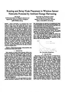
MRA IMA STPA GMA EGMA
2
1.5
34
33
32 1
2000
2500 3000 3500 Maximum Movement (m)
4000
4500
5000
Total relay movement, varying R, N = 20, k = 2
for the number of relays they require and the movement of the existing relays. We study the performance of the algorithms for different values of R, and different number of terminal nodes (N ) in the network. The matching algorithm used was an implementation of Gabow’s N-cubed weighted matching algorithm [11]. 1) Variation with movement of terminals: We first fixed the number of terminal nodes (N ) at 20, and varied the amount of movement of the terminal nodes. The network was formed with 10 different randomly generated node locations, and for each set of node locations, 10 different sets of node movements were generated. Thus, the algorithms were run a total of 100 times. The first set of results are for achieving 2-edge connectivity among the terminal nodes. The maximum movement allowed (R) for each node was varied from 500m to 5km. Figure 1 shows the average total distance moved by existing relays in MRA, IMA, STPA, GMA and EGMA. Figure 2 shows the average total number of relays required in the new topology formed by MRA, IMA, STPA, GMA and EGMA. STPA and EGMA work better than GMA and IMA, which in turn work better than MRA in terms of the total relay movement. MRA saves only a few relays compared to the other methods. This savings is offset by the larger movement distance it requires. STPA works slightly better than EGMA when the terminal nodes do not move much, whereas EGMA works much better than STPA as the terminal movement increases. This is expected as STPA tries to move the existing relays to connect the same terminal pair they were associated with before, and thus works well for small terminal node movements. For large movements, EGMA works better as the terminals may move quite far from their original locations and thus it may be better to move existing relays to connect terminal nodes other than the ones they were associated with before. Figures 3 and 4 show the ratio between EGMA and MRA of distance moved by relays and of total number of relays required. EGMA leads to a savings of 20% in the distance travelled by existing relays on an average, for all values of R. Also, the number of relays required by EGMA is almost the same as in MRA on an average. It is worthwhile to note
30 500
Fig. 2.
1000
1500
2000
2500 3000 3500 Maximum Movement (m)
4000
4500
5000
Number of relays needed, varying R, N = 20, k = 2
2 EGMA 1.8
1.6
1.4 Relative Total Distance
1500
1.2
1
0.8
0.6
0.4
0.2 500
1000
1500
2000
2500 3000 3500 Maximum Movement (m)
4000
4500
5000
Fig. 3. Total relative relay movement in EGMA, varying R, N = 20, k = 2
1.4
1.3
1.2 Relative Total Relays Needed
Fig. 1.
1000
31
1.1
1
0.9
0.8
EGMA 0.7 500
Fig. 4.
1000
1500
2000
2500 3000 3500 Maximum Movement (m)
4000
4500
5000
Relative number of relays in EGMA, varying R, N = 20, k = 2
2 STPA 1.8
1.6
1.4 Relative Total Distance
0.5 500
MRA IMA STPA GMA EGMA
1.2
1
0.8
0.6
0.4
0.2 500
1000
1500 Maximum Movement (m)
2000
2500
Fig. 5. Total relative relay movement in STPA, varying R, N = 20, k = 3
1.35
1.5 STPA
1.3
1.4 1.25
Relative Total Relays Needed
Relative Total Relays Needed
1.3 1.2
1.15
1.1
1.05
1
1.2
1.1
1
0.9 0.95
0.8
0.9
STPA
0.85 500
Fig. 6.
1000
1500 Maximum Movement (m)
2000
0.7 10
2500
Relative number of relays in STPA, varying R, N = 20, k = 3
Fig. 8.
15
20
25
30 35 Number of Terminals
40
45
50
Relative number of relays in STPA, varying N , R = 1500, k = 2
1.8 STPA
very high, then EGMA performs better than STPA (and all other algorithms), and thus should be used in those cases.
1.6
Relative Total Distance
1.4
1.2
V. C ONCLUSION
1
0.8
0.6
0.4
0.2 10
Fig. 7. k=2
15
20
25
30 35 Number of Terminals
40
45
50
Total relative relay movement in STPA, varying N , R = 1500,
than in some instances MRA may require more relays because the algorithm for finding a minimum-relay k-edge connected topology is not optimal. Thus, other algorithms may use less relays than MRA in some instances, though that is not true on an average (as the results show). We also simulated MRA and STPA (it works as well as EGMA for the values of R used) for the objective of constructing a 3-edge connected topology. The number of simulations were the same as before. Figures 5 and 6 show the ratio between STPA and MRA of distance moved by relays and of total number of relays required. STPA leads to a savings of 20-25% in total relay movement on an average for varying values of R for k = 3 as well. Also, the number of relays used is almost the same as in MRA on an average. 2) Variation with number of terminals: We now study the variation with respect to the number of terminal nodes in the network. The simulation set up is the same as before, and they are done on 10 sets of network locations with 10 sets of random movements. The objective is to construct a 2-edge connected topology among the terminal nodes. The maximum movement allowed (R) for each node is fixed at 1500m. Figures 7 and 8 show the ratio between STPA and MRA of distance moved by relays and of total number of relays required. STPA leads to about 15-20% less movement of existing relays than MRA, and uses almost the same number of relays on an average for all values of N considered. Thus, STPA works much better than MRA for a wide range of number of terminals and amount of movement of terminal nodes (R). If the amount of terminal movement is
This paper considers the problem of providing faulttolerance to nodes in an ad-hoc network with low mobility. The tolerance is provided against node and link failures. We use additional relay nodes for construction of a fault-tolerant topology due to transmission range constraints. We provide algorithms for construction of a topology tolerant against the desired number of failures, using as few relays as possible. The algorithms re-establish the topology when it is disrupted due to node movement, and try to minimize the distance travelled by relays in the network, thus re-establishing it quickly. We do extensive simulations to show that the proposed algorithms lead to significant savings in the distance travelled by relays (while using almost the same number of relays) compared to an algorithm that only tries to minimize the number of relays. The algorithms are shown to work well with varying amount of terminal movement and varying number of network nodes. R EFERENCES [1] E. Perkins, Ad Hoc Networking. Addison-Wesley, 2001. [2] K. Xu, X. Hong, and M. Gerla, “An ad hoc network with mobile backbones,” IEEE ICC, vol. 5, pp. 3138–3143, 2002. [3] P. Basu and J. Redi, “Movement control algorithms for realization of fault-tolerant ad hoc robot networks,” IEEE Network, pp. 36–44, July/August, 2004. [4] A. Kashyap, S. Khuller, and M. Shayman, “Relay placement for higher order connectivity in wireless sensor networks,” IEEE INFOCOM, 2006. [5] S. Khuller and U. Vishkin, “Biconnectivity approximations and graph carvings,” Journal of the ACM, vol. 41, no. 2, pp. 214–235, 1994. [6] S. Khuller and B. Raghavachari, “Improved approximation algorithms for uniform connectivity problems,” Journal of Algorithms, vol. 21, no. 2, pp. 434–450, 1996. [7] V. Auletta, Y. Dinitz, Z. Nutov, and D. Parente, “A 2-approximation algorithm for finding an optimum 3-vertex connected spanning subgraph,” Journal of Algorithms, vol. 32, pp. 21–30, 1999. [8] Y. Dinitz and Z. Nutov, “A 3-approximation algorithm for finding optimum 4,5-vertex connected spanning subgraphs,” Journal of Algorithms, vol. 32, pp. 31–40, 1999. [9] G. Kortsarz and Z. Nutov, “Approximating node connectivity problems via set covers,” Algorithmica, vol. 37, pp. 75–92, 2003. [10] L. Lov´asz and M. D. Plummer, Matching Theory. North-Holland, 1986. [11] H. Gabow, “Implementation of algorithms for maximum matching on nonbipartite graphs,” Ph.D. thesis, Stanford University, 1973.