Reliable Attribute Selection based on Random forest(RASER) Aboudi Noura
Hechmi Shili
Lotfi Ben Romdhane
Department of Computer Science University of Monastir
[email protected]
Department of Computer Science University of Monastir
[email protected]
Department of Computer Science University of Sousse
[email protected]
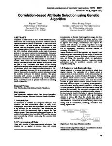
Abstract—Feature selection has become one of the most active research areas in the field of data mining. It allows removing redundant and irrelevant data sets of large size. Furthermore, there are several methods in the literature for selecting attributes. In this article, a new multi-objective method is proposed to select relevant and non-redundant features. Our proposed feature selection method is divided into three stages: The first step computes the feature relevance value based on random forests. The second step, computes the dissimilarity matrix representing the dependence between the features of our training datasets, and transform it into a complete graph whose nodes represent features and edges represent the values of dissimilarities between them. The last step is for the optimization in which a multi-objective optimization algorithm is applied. The proposed method is applied on many datasets to find the most relevant and non-redundant features and the performance of the proposed method is compared with that of the popular MBEGA, mRMR (MIQ) and mRMR (MID).
Figure 1: General feature selection process[3] Generally, a typical feature selection method illustrated in Fig. 1, consists of four components: a subset generation or search procedure, an evaluation function, a stopping criterion, and a validation procedure[3]. The selection of attributes will be based on two criteria: relevance and redundancy. Definition 1. Relevance: In the literature, there are several definitions of the concept of relevance of a feature, the best known is that of ([4],[5]). A feature fi is said relevant if its absence reduces significantly the performance of the used classification system. Definition 2. Redundancy: The notion of redundancy is relatively associated with correlation function. So, we say that two attributes are redundant if their values are completely correlated [6]. The concept of redundancy will be defined with the Markov blanket [7]. If G be a set of attributes, an attribute is redundant and can be removed from G if it is not relevant and Markov blanket M in G. According to the property of Markov blanket, it is easy to
Keywords: feature selection; feature relevance; feature redundanc; multi-objective optimization; random forest
I.
INTRODUCTION
Feature selection is a problem that has to be addressed in many areas. The resolution of general problems is based on the treatment of features[1]. So the performance of the treatment system depends on the correct selection of features: considering many features increases the risk of considering redundant and irrelevant features. Therefore, it is necessary to use a method for reducing the data size. The feature selection identify a subset of attributes of minimal size necessary and sufficient to define the target concept[2].
1
see that a redundant attribute remains removed redundant when other attributes are removed. II.
find a subset of variables that maximizes the objective function which is the classification performance[14].
RELATED WORK
III.
In the literature, feature selection methods are generally grouped into three categories: filter, wrapper and embedded approaches [8]. The filter approach uses statistical measures calculated to filter characteristics according to the number of criteria. This step is generally carried out before applying any classification algorithm[8]. In filter approach, there are several methods such as minimal and redundancy-maximal-relevance criterion (mRMR)[9]. The mRMR is a screening method for the selection of attributes who have the best interests of the target class, are a little redundant and most dissimilar to each other. This method is based on statistical measures such as mutual information, correlation criteria, etc. The two optimization criteria (maximum relevance (MR) and minimum redundancy (mR)) are based on mutual information[10]. There are two types of mRMR that is different depending on the combination of the two criteria(addition and : mRMR(MID) and mRMR(MIQ). mRMR(MID)= max(Pertinence - Redundancy)
(1)
mRMR(MID)= max(Pertinence / Redundancy)
(2)
RELIABLE ATTRIBUTE SELECTION BASED ON RANDOM FOREST(RASER)
The feature selection is applied to reduce the number of attributes in many applications. Most features selection methods mainly focus on finding the relevant features[15]. We show that the notion of relevance is not sufficient for effective selection of high-dimensional data because of the high correlation that may exist between different features. In many problems, there exist different aspects of solutions which are partially or wholly in conflict. Therefore, treating these problems as single objective optimization produces an unreliable result. In multi-objective optimization problem the objectives may estimate those different aspects of solutions which are conflicting in nature. After defining the problem of multi-objective optimization, meta heuristics are designed to solve the multi-objective problems. The goal of a multiobjective optimization is to identify a set of solutions in the Pareto optimal set [6]. This section is devoted to the explanation of our contribution, which is to propose a new method for the selection of relevant non-redundant features on the basis of the random forests method. Our method is divided into three steps. The approach followed is recapitulated in Fig.2.
Besides, there are many other methods such as: Correlation based on feature selection (CFS), Markov blanket filter (MBF)... The wrapper methods on the contrary, use induction algorithm to evaluate the candidate feature subsets. They generally select feature subsets more suitable for the induction algorithm than the filter methods. In wrapper approach, there are several methods such as:Markov blanket-embedded Genetic Algorithm( MBEGA)[3] provided by Zexuan and Al in the selection of genes. MBEGA used Markov blanket to narrow the search by adding some relevant attributes or removing redundant and/or irrelevant attributes in the solutions selected by genetic algorithm (GA). The embedded feature selection method, similar to wrapper methods and the feature selection is linked to the classification stage. The embedded methods have been proposed to reduce the classification of learning. They try to combine the advantages of both previous methods. The learning algorithm takes advantage of its own variable selection algorithm. See for example: PLSRFE [11], RF-RFE[12]. Most of the traditional feature selection methods define some metrics to evaluate each individual feature, such as signal-tonoise ratio (SNR)[6] and information gain[13]. They also use many statistical hypotheses testing techniques such as parametric t-test , F-test [11] . Since evaluating subsets becomes an NP-hard problem, suboptimal subsets are found by using search algorithms that find a subset heuristically. A number of search algorithms can be used to
Figure 2:The steps of our model
First, we compute the relevance values of each feature using random forests. In the second step, we compute the dissimilarity matrix from our training set by using the
2
correlation criterion. Then, our problem is represented by a complete graph whose nodes represent the attributes and the edges represent the value of dissimilarity between them.
study examines the effectiveness of variable importance measures by random forests in identifying the true indicator of a large number of candidate predictors. Random forests provide an original way for calculating the relevance value of feature. Random forest consists of a number of decision trees. Every node in the decision trees is a condition on a single feature. So, in a random forest or each node of the tree represents an atttribute. Random forests handle the problem of relevance but not the problem of redundancy. Therefore, we will use the graph dissimilarity to handle features redundancy. Algorithm 1 is used for computing of the relevance value [16].
The last step is the optimization step in which we apply a multi-objective optimization algorithm (relevance, redundancy) on the dissimilarity graph to obtain an optimal subgraph embedding the most relevant non-redundant features. A. Measuring features relevance Random forests do not require the reduction of the prediction space before classification. In addition, random forests measure the relevance of features for each predictor candidate[16]. This
an attribute and each edge between two attributes represents the relationship between them. For a set A of N attributes where A = { ; ; ;…; }, the arrangement of the training set may be considered as a twodimensional matrix where the columns represent the attributes and rows represent instances attributes.
Measuring redundancy The feature selection process is represented by the graphs, whether G = (V; E) a graph constructed by a set of nodes V and a set of edges E V ×V ; and W is a weight matrix whose values are in the range [0:1]. Each node of the graph represents
3
There are a variety of methods for measuring of similarity dissimilarity between the attributes such as: Euclidean distance, correlation coefficient [6], etc. By using one of these dissimilarity measures a symmetric matrix is generated called dissimilarity matrix. Therefore if we have a set of attributes A = { ; ; ;…; }, computation of dissimilarity between attributes is handled by a (n×n). The dissimilarity matrix is computed from the data matrix by using the correlation coefficient [1] between each pair of attributes. The correlation coefficient σ between two random attributes x and y is defined by: (
)
( √
( )
) ( )
Figure 3: Example of subgraph extration
The problem of finding the subgraph is an NP-hard problem[1]. To solve our problem we will use multi-objective optimization algorithm graph based MbPSO [6], which is described by the algorithm 2. In multi-objective optimization problem the objectives may estimate those different aspects of solutions which are conflicting in nature [6].
(3)
Where ( ) denotes the variance of a variable and ( )the covariance between two variables. If x and y are completely correlated (i.e., there is a linear dependency), then σ(x, y) is 1 or -1. If they are totally uncorrelated then σ (x; y) is 0. Hence equation (4) represents the dissimilarity between x and y. (
| (
)|)
The algorithm 3 describes the different steps of our proposed new method cited above.
(4)
Subsequently, according to the dissimilarity matrix a weighted complete graph G is formed. The value at row i and column j in the dissimilarity matrix , represents the weight of the edge between node and . As each feature has some dissimilarity value with other features (present in dissimilarity symmetric matrix ), hence the graph G is a complete graph. Now our problem is how to determine the optimal number of relevant and non-redundant attributes. So, we have to select an optimal subgraph g of G that contains the most relevant attributes and non-redundant. Therefore, we will apply the algorithm Multi-objective Binary PSO based Approach [6] as explained subsequently. Subgraph computation The problem of finding the most relevant and non-redundant attributes is modeled by finding the optimal subgraph from a weighted undirected graph. The attributes contained by the extracted subgraph comprise the final selected relevant and non-redundant features. Figure 3 is an example, that the left graph is the initial graph that contains 5 nodes and value of sij is the dissimilarity value between attributes and each attribute has a relevance value Ri. The sub-graph on the right is the returned after the application of the optimization algorithm.
4
5
IV.
It is based on estimated performance from examples that were not used in the design of the model. The cross-validation algorithm k -fold cut the initial set of D examples in k blocks. The cross-validation algorithm is described in [1]. The performance of our proposed method RASER is compared with: MBEGA[3], mRMR(MID)[9], mRMR(MIQ)[9] methods. The datasets are arbitrarily divided into two groups: all together for learning and for testing. Each algorithm is executed for each training set and evaluated by the appropriate test portion. The performance analysis is extended using 10-fold cross validation. The all algorithms are executed on the total sample versus datasets and the output features are validated using 10-fold cross-validation using Support Vector Machine (SVM).
EXPERIMENTAL RESULTS
In this section, we first describe the datasets, their preprocessing procedure and the performance metrics followed by the results of different algorithms. In this article nine datasets are used which are publicly available from[1]. Table I summarizes these datasets. The first column reports the datasets name, the second column the number of features and the third column the number of instances. The final column reports the number of classes as well as the size of each class. For example, the WBC dataset is composed of 699 instances described each by 10 features. It is composed of two classes (458 Benign, 241 Malignant). Performance is evaluated using sensitivity, specificity, accuracy and error-rate. Sensitivity =
(5)
Specificity =
(6)
Errorrate =
(7)
Accuracy =
(8)
A. Value of relevance To compute the features relevance value, we applied the random forest method that contains ntree trees. The figure 4 shows the influence on the choice of ntree value relevance. We can see in figure 4 that the number of trees (ntree) has practically no effect on the relevance. So for our work, we choose 200 as ntree value, that is, each built forest contains 200 trees. Figure 5 show the relevance of attribute values for the WPBC dataset.
Where TP: True Positive= correctly identified TN: True Negative= correctly rejected FP: False Positive= incorrectly identified FN: False Negative= incorrectly rejected As this evaluate our method, it is necessary to use a datasets that were not used for learning: this is what is called the test datasets. It contains also labeled examples to compare the predictions of a hypothesis with the actual value of the class. This test is generally achieved by reserving part of the initial supervised examples and that will not be used in the learning phase. Crossvalidation is a method of estimating reliability of a model based on a sampling technique. Figure 4: Influence of ntree on value of relevance for WBC datasets TABLE I.
DESCRIPTION OF THE USED DATASETS
Dataset name WBC WPBC
#Features
#Instances
10 34
699 198
WDBC Spambase Ionosphere Madelon Dermatology
32 57 34 500 33
569 4601 351 4400 366
#Classes 2 (458 Benign, 241 Malignant) 2(151 non-récurrent, 47 récurrent) 2(357 benign, 212 malignant) 2(spam, not spam) 2(good, bad) 2 6(112 psoriasis, 61 seboreic dermatitis, 72 lichen planus, 49 pityriasis rosea, 52 cronic dermatitis, 20 pityriasis rubra pilaris) Figure 5: Attributes relevance value of WPBC datasets
6
B.
Performance
the sensitivity, specificity, accuracy, and errorrate values of our model are better than mRMR(MID) mRMR(MIQ) and
In Table II we compare the classification results obtained with the original dataset that contains all the attributes and the dataset that contains the attributes selected by our method. We note that our algorithm, in general returns a classification rate higher than that returned by the classification of the original dataset.
MBEGA. The average Accuracy for our method is very much upper than other methods i.e. proposed method results are more non-redundant and relevant features than other comparative methods.
The cross-validation scores of different algorithms are reported in Table III. It is clear from this table for the most of datasets TABLE II.
Dataset
COMPARISONS OF THE CLASSIFICATIONS RESULTS
Methods
Specificity (%)
Sensitivity (%)
% Accuracy
% Error rate
RASER
98
97.3
97.6
2.4
Original classification
97
96.1
96.4
3.6
RASER
88.1
96.1
93.4
6.5
Original classification
55.3
78.1
76
24
RASER
97.6
95.5
96.2
3.7
Original classification
95.7
96.9
96.5
3.4
RASER
95.5
98.3
97.2
2.7
Original classification
93.3
96.5
95.3
4.7
RASER
34
98
74
26
Original classification
1
100
61
34
RASER
96
97
96
3
Original classification
52
66
64
36
RASER
99
100
95
5
Original classification
100
98
89
10
RASER
51
46
50
50
Original classification
50
47
48
52
WBC BC
WPBC
WDBC
Spambase
Ionosphere
Dermatology
Madelon
7
TABLE III.
Dataset
COMPARISONS OF THE CLASSIFICATIONS RESULTS WITH OTHER FEATURE SELECTION ALGORITHMS
Specificity (%)
Sensitivity (%)
% Accuracy
% Error rate
RASER
98
97.3
97.6
2.4
MBEGA
95.9
97.6
96.9
3.1
mRMR(MID)
92
91.3
91.5
8.4
mRMR(MIQ)
90.8
96.7
94.6
5.3
RASER
88.1
96.1
93.4
6.5
MBEGA
45.5
82.3
71.3
28.7
mRMR(MID)
57.3
73.8
69.8
30.1
mRMR(MIQ)
65.5
70.1
70.2
29.7
RASER
97.6
95.5
96.2
3.7
MBEGA
68.2
73.2
72.7
27.2
mRMR(MID)
60.8
72.9
71.1
28.9
mRMR(MIQ)
66.9
75.1
73.8
26.1
RASER
95.5
98.3
97.2
2.7
MBEGA
90.9
98.8
95.7
4.3
mRMR(MID)
92.7
95.1
94.1
5.8
mRMR(MIQ)
92.2
96.3
94.7
5.2
RASER
34
98
74
26
MBEGA
10
99
64
35
mRMR(MID)
65
35
61
38
mRMR(MIQ)
66
38
62
37
RASER
96
97
96
3
MBEGA
81
21
73
27
mRMR(MID)
65
38
61
38
mRMR(MIQ)
47
24
75
84
RASER
99
100
95
5
MBEGA
100
97
90
10
mRMR(MID)
97
96
81
18
mRMR(MIQ)
98
96
93
6
RASER
51
46
50
50
MBEGA
38
57
54
46
mRMR(MID)
5
54
0.53
47
mRMR(MIQ)
49
51
50
50
Methods
WBC
BC
WPBC
WDBC
Spambase
Ionosphere
Dermatology
Madelon
8
V.
application aux données de biopuces, Journal de la société française de statistique 149 (3) (2008) 43–66. [17] ] M. B. Eisen, P. T. Spellman, P. O. Brown, D. Botstein, Cluster analysis and display of genomewide expression patterns, Proceedings of the National Academy of Sciences 95 (25) (1998) 14863–14868. [18] P. Crescenzi, V. Kann, M. Halldórsson, A compendium of np optimization problems (1995). [19] https://archive.ics.uci.edu/ml/datasets.html
CONCLUSION
In this paper, we have proposed a novel feature selection algorithm based on random forest to select the most relevant and non-redundant one. In that purpose, we have used the random forest method to measure the relevance value attributes and the correlation coefficient to calculate the value of redundancy. The proposed method is performed in three basic steps three stages: the measure of relevance of attributes, modeling and optimization. Finally, we tested our approach for the selection of attributes on datasets and we have approved its effectiveness. These encouraging results should stimulate future research. Our immediate concern is to use another measures of dissimilarity criterion.
.
REFERENCES [1]
[2]
[3]
M. L. SAMB, F. CAMARA, S. NDIAYE, Y. SLIMANI, M. A. ESSEGHIR, Approche de sélection d’attributs pour la classification basée sur l’algorithme rfe-svm. H. CHOUAIB, Sélection de caractéristiques:méthodes et applications, 2011.URL : http://www.math-info.univparis5.fr/~vincent/siten/Publications/theses/pdf/chouaib.pdf Z. Zhu, Y.-S. Ong, M. Dash, Markov blanket-embedded genetic algorithm for gene selection, Pattern Recognition 40 (2007) 3236 – 3248. URL:http://www.sciencedirect.com/science/article/pii/S003132030 7000945
[4]
George, H. (1997). John. Enhancements to the data mining process (Doctoral dissertation, Ph. D thesis of Stanford University).
[5]
K. R. P. K. John, G. H., Irrelevant features and the subset selection problem (1994) 121–129. M. Mandal, A. Mukhopadhyay, A graph-theoretic approach for identifying non-redundant and relevant gene markers from microarray data using multiobjective binary pso, PloS one 9 (3) (2014) e90949. D. Koller, M. Sahami, Toward optimal feature selection (1996) 284–292. Y. Saeys, I. Inza, P. Larrañaga, A review of feature selection techniques in bioinformatics, bioinformatics 23 (19) (2007) 2507– 2517. H. Peng, F. Long, C. Ding, Feature selection based on mutual information criteria of maxdependency, max-relevance, and minredundancy, Pattern Analysis and Machine Intelligence, IEEE Transactions on 27 (8) (2005) 1226–1238. B. R, Using mutual information for selecting features in supervised neural net learning, IEEE Trans Neural Network. W. You, Z. Yang, G. Ji, Pls-based recursive feature elimination for high-dimensional small sample, Knowledge-Based Systems 55 (2014) 15–28. Q. Zhou, H. Zhou, Q. Zhou, F. Yang, L. Luo, Structure damage detection based on random forest recursive feature elimination, Mechanical Systems and Signal Processing 46 (1) (2014) 82–90. B. Azhagusundari, A. S. Thanamani, Feature selection based on information gain, International Journal of Innovative Technology and Exploring Engineering (IJITEE) ISSN (2013) 2278–3075. G. Chandrashekar, F. Sahin, A survey on feature selection methods, Computers & Electrical Engineering 40 (1) (2014) 16– 28. L. Yu, H. Liu, Feature selection for high-dimensional data: A fast correlation-based filter solution, in: ICML, Vol. 3, 2003, pp. 856– 863. B. Ghattas, A. B. Ishak, Sélection de variables pour la classification binaire en grande dimension: comparaisons et
[6]
[7] [8]
[9]
[10] [11]
[12]
[13]
[14]
[15]
[16]
9