[22] proposes a tracking algorithm using adaptive random forests for real- .... using the R software for statistical computing (http://www.r-project.org/). .... significance level of 5%; average rank of each value of minNum and the percentage of.
Root Attribute Behavior within a Random Forest Thais Mayumi Oshiro and Jos´e Augusto Baranauskas Department of Computer Science and Mathematics, Faculty of Philosophy, Sciences and Languages at Ribeirao Preto, University of Sao Paulo, Brazil {thaismayumi,augusto}@usp.br
Abstract. Random Forest is a computationally efficient technique that can operate quickly over large datasets. It has been used in many recent research projects and real-world applications in diverse domains. However, the associated literature provides few information about what happens in the trees within a Random Forest. The research reported here analyzes the frequency that an attribute appears in the root node in a Random Forest in order to find out if it uses all attributes with equal frequency or if there is some of them most used. Additionally, we have also analyzed the estimated out-of-bag error of the trees aiming to check if the most used attributes present a good performance. Furthermore, we have analyzed if the use of pre-pruning could influence the performance of the Random Forest using out-of-bag errors. Our main conclusions are that the frequency of the attributes in the root node has an exponential behavior. In addition, the use of the estimated out-of-bag error can help to find relevant attributes within the forest. Concerning to the use of pre-pruning, it was observed the execution time can be faster, without significant loss of performance. Keywords: Machine Learning, Random Forest.
1
Introduction
A great interest in the machine learning research concerns ensemble learning — methods that generate many classifiers and combine their results. It is largely accepted the performance of a set of many weak classifiers is usually better than a single classifier given the same quantity of train information [21]. Ensemble methods widely known are boosting [11,23] and bagging [6], and more recently Random Forests [5,16]. In the bagging method (bootstrap aggregation), different training subsets are randomly drawn with replacement from the entire training set. Each training subset is fed as input to base learners. All extracted learners are combined using a majority vote. While bagging can generate classifiers in parallel, boosting generates them sequentially. Random Forests is another ensemble method, which constructs many decision trees that will be used to classify a new instance by the majority vote. Each split H. Yin et al. (Eds.): IDEAL 2012, LNCS 7435, pp. 733–742, 2012. c Springer-Verlag Berlin Heidelberg 2012 �
734
T.M. Oshiro and J.A. Baranauskas
of the decision tree uses a subset of attributes randomly selected from the whole original set of attributes. Additionally, each tree uses a different bootstrap sample of the data in the same manner as bagging. Normally, bagging is more accurate than a single classifier, but it is sometimes much less accurate than boosting. On the other hand, boosting can create ensembles that are less accurate than a single classifier. In some situations, boosting can overfit noisy datasets, thus decreasing its performance. Random Forests, on the other hand, are more robust than boosting with respect to noise; faster than bagging and boosting; its performance is as good as boosting and sometimes better, and they do not overfit [5]. Nowadays, Random Forest is a method of ensemble learning widely used in the literature and applied fields. But the associate literature provides few information about what happens in the trees within the Random Forest. This study tries to provide insights about what happens at the root level of Random Forests. We have analyzed the frequencies of all attributes in trees at root level. In addition, aiming to find out if these attributes were good ones and if there is a best attribute among the top ten, we have used an estimated out-of-bag error as a supplementary metric. This metric enables to differentiate attributes that had the same frequency, and thus, may identify the best attribute used by a tree in the root node. Biomedical datasets are characterized by fairly few instances and many attributes. Irrelevant attributes not only lead to low performance, but also add extra difficulties in finding potentially useful knowledge [18,20]. Therefore, excluding irrelevant attributes facilitates the data visualization and may improve the classification performance. In addition, identifying a subset or a single best attribute in a biomedical dataset can improve human knowledge. Even Random Forests are being widely used, we did not find any similar work to this one in the literature and thus, this work can provide new insights that may help future works and researches. Even considering there is no similar work to this one, we preset in the next section some recent researches using Random Forests. The remaining of this paper is organized as follows. Section 2 describes some related work. Section 3 describes what Random Tree and Random Forest are and how they work. The datasets used in the experiments are described in Section 4 and Section 5 describes the experimental methodology used and the results of the experiments are shown in Section 6. Section 7 presents the conclusions.
2
Related Work
Since Random Forests are efficient, multi-class, and able to handle large attribute space, they have been widely used in several domains such as real-time face recognition [22], bioinformatics [13] and there are also some recent research in medical domain, for instance [15] as well as medical image segmentation [24]. [22] proposes a tracking algorithm using adaptive random forests for realtime face tracking and the approach was equally applicable to tracking any
Root Attribute Behavior within a Random Forest
735
moving object. [13] presents one of the first illustrations of successfully analyzing genome-wide association (GWA) data with a machine learning algorithm (Random Forests). In [15] they introduce an efficient keyword based medical image retrieval method using image classification with Random Forests classifier and confidence assigning of each keyword. [24] proposes an enhancement of the Random Forests to segment 3D objects in different 3D medical imaging modalities.
3
Random Trees and Random Forests
Assume a training set T with a attributes and n instances and define Tk a bootstrap training set sampled from T with replacement, containing n instances and using m random attributes (m ≤ a) at each node. A Random Tree is a tree drawn at random from a set of possible trees, with m random attributes at each node. The term “at random” means that each tree has an equal chance of being sampled. Random Trees can be efficiently generated, and the combination of large sets of Random Trees generally leads to accurate models [25,9]. A Random Forest is defined formally as follows [5]: it is a classifier consisting of a collection of L Random Tree classifiers {hk (x, Tk )}, k = 1, 2, . . . , L, where Tk are independent identically distributed random samples and each tree casts a unit vote for the most popular class at input x. As already mentioned, Random Forests employ the same method bagging does to produce random samples of training sets (bootstraps samples) for each Random Tree. Each new training set is built, with replacement, from the original training set. Thus, the tree is built using the new subset and a random attribute selection. The best split on the random attributes selected is used to split the node. The trees grown are not pruned. In a Random Forest, the out-of-bag method works as follows: given a specific training set T , generate bootstrap training sets Tk , construct classifiers {hk (x, Tk )} and let them vote to create the bagged classifier. For each (x, y) in the training set, aggregate the votes only over those classifiers for which Tk does not contain (x, y). This is the out-of-bag classifier. Then the out-of-bag estimate for the generalization error is the error rate of the out-of-bag classifier on the training set [5].
4
Datasets
The experiments reported here used 14 datasets (with 2 variants), all representing real medical data and none of which had missing values for the class attribute. The biomedical domain is of particular interest since it allows one to evaluate Random Forests under real and difficult situations often faced by human experts. A brief description of each dataset is provided. Lung Cancer, CNS (Central Nervous System Tumour Outcome), Lymphoma, Ovarian 61902, Leukemia, Leukemia nom., and WDBC (Wisconsin Diagnostic
736
T.M. Oshiro and J.A. Baranauskas
Breast Cancer) are all related to cancer and their attributes consist of clinical, laboratory and gene expression data. Leukemia and Leukemia nom. represent the same data, but the second one had its attributes discretized [17]. C. Arrhythmia (C. stands for Cardiac) is related to heart diseases and its attributes represent clinical and laboratory data. Allhyper, Allhypo, Sick and Thyroid 0387 are a series of datasets related to thyroid conditions. Dermatology is related to human conditions. Datasets were obtained from the UCI Repository [10], except CNS and Lymphoma were obtained from [2]; Ovarian 61902 was obtained from [3]; Leukemia and Leukemia nom. were obtained from [1].
5
Experimental Methodology
In a previous work [19], it was analyzed an optimal range for the number of trees within a Random Forest, i.e., a threshold from which increasing the number of trees would bring no significant performance gain, and would only increase the computational cost. We found, based on the performed experiments, that a range between 64 and 128 trees in a forest is the most indicated for accuracy estimation. Under this situation, we have tried to generate forests containing 128 trees but without stability on the experiments reported in the next section. In this case, we assume that a result (10 top attributes subset) is stable when increasing the number of trees there is almost no change in the subset (the 10 top attributes remain basically the same). Denote αL the subset of the 10 most important attributes obtained from L Random Trees (see in Section 6 how the subsets were obtained). Then, we define attributes subset stability using L Random Trees as |αL ∩ α2L | � 10. First, we have used 64 and 128 trees in datasets with many attributes, and it was observed that the subsets of the 10 top attributes varied widely. We have also tried a2 trees, again without stability, where a is the number of attributes in the dataset. Finally, forests containing a and 2a trees presented stable results that are reported in this text. The lesson that can be learnt from the previous and the current experiments is that nice accuracy can be reached rapidly with 64–128 trees; this point-of-view sees the random forest as a black-box. However, looking specific factors inside a random forest, i.e. looking the random forest as a white-box, may require more trees. To assess performance, 10-fold cross-validation was performed in the experiments. All experiments refer to the position of the attribute (i.e., the index of the attribute in the dataset according to Weka [14], which starts at zero) as its ID. In order to analyze if some results were significantly different, we applied the Friedman test [12], considering a significance level of 5%. If the Friedman test rejects the null hypothesis, a post-hoc test is necessary to check in which classifier pairs the differences actually are significant [8]. The post-hoc test used was the Benjamini-Hochberg [4] and we performed an all versus all comparison, making all possible comparisons among the twelve forests. The tests were performed using the R software for statistical computing (http://www.r-project.org/).
Root Attribute Behavior within a Random Forest
6
737
Experiments, Results and Discussion
Experiment 1. In this experiment we have looked for the average attribute frequency at root level, for instance, if attributes appear uniformly or if there is a subset of them that is most commonly used. To perform this experiment, two measures were used: the number of times an attribute was among the m random attributes selected by the tree at the root level (timesSelected) and the number of times this attribute was, in fact, chosen to be at the root node (timesRoot). Then we have used the ratio between them (F requency = timesRoot/timesSelected) to analyze attribute frequency. After sorting frequencies for all attributes in each dataset, it is possible to note they present an exponential behavior. In Figure 1 is shown this exponential behavior using the dataset C. Arrhythmia. The other datasets present similar behaviors, and thus, these figures were omitted. In Figure 2 only the ten highest frequencies are shown in order to facilitate the analysis. There are four lines in each graphic representing the mean and median frequencies for forests using a and 2a trees (ordered by the mean frequencies of the forest using a trees). From this figure, it is possible to observe in some cases there is a single attribute that stands out (for instance, Allhyper and Allhypo both containing few attributes), and in other cases there is a subset of attributes most often used (for instance, Lymphoma and Leukemia, both containing a large number of attributes).
(a) Using a trees
(b) Using 2a trees
Fig. 1. Frequency of all attributes using the dataset C. Arrhythmia
Experiment 2. Now suppose there are three attributes in the best attribute subset, A, B and C. Assume all of them have the same frequency, but attribute A has estimated out-of-bag error equals to 0.90, B equals to 0.65 and C equals to 0.20. In this case, we assume attribute C is the best one in the subset, since its performance is the best. The question that arises is how to estimate the out-of-bag error for a given attribute. The root level attribute represents the most important condition for classes discrimination [7] in the tree, and therefore, one can assume it determines the performance of the tree itself. Under this assumption we have used the out-of-bag error of the tree when attribute α is at its root level as an estimate of performance for attribute α. With this modifications, we have performed a second experiment, in which frequencies have been altered to F requency × (1 − OOB), where OOB corresponds to the mean out-of-bag error of an attribute as explained before. The results of this experiment are shown in Figure 3.
738
T.M. Oshiro and J.A. Baranauskas
Fig. 2. Frequency of the 10 most used attributes in all datasets. The x-axis corresponds to the number of the attribute and the y-axis corresponds to the frequency. Although all y-axis ranges from 0 to 1, this interval varies in some graphics for better viewing.
Analyzing the results, it can be observed that in all datasets the frequency had an exponential behavior or similar, even in the datasets that showed a linear behavior in the first experiment. Thus, using the estimated out-of-bag error there is mostly only one attribute that stands out in each dataset. Experiment 3. As mentioned earlier, Random Forests do not overfit, although trees within them are grown without post-pruning. In this experiment we have analyzed the behavior of pre-pruning, since it can speed up Random Forest induction. To perform pre-pruning of the trees of the Random Forest, the parameter minN um was used. It determines the minimum total weight of the instances in a leaf, where the default value in Weka [14] is 1.0, generating very large trees. Based on this, we have used ten different values of minN um: 1, 2, 3, 5, 7, 11, 13, 17, 19 and 23. As explained before, for accuracy estimation a range from 64–128 trees are enough [19]. Based on this result, we have built forests with 128 trees in this experiment. To analyze the several values of minN um we have used AUC values and we have applied the Friedman test [12], considering a significance level of 5%. In addition, we have observed the average execution time to induce the forest using each different value of minN um. This measure was taken based on the average execution time to induce the forest using minN um = 1, i.e, the execution time to induce this forest was taken as 100% and the remaining percentages were calculated based on this one, since for large values of minN um the time is shorter, due to the pre-pruning process that stops the growth of trees. Table 1 presents the results of the post-hoc test after the Friedman’s test and the rejection of the null hypothesis, the average rank and the percentage of the average execution time of each value of minN um. In this table � (�) indicates the Random Forest at the specified row is better (significantly) than the Random Forest at the specified column; � (�) the Random Forest at the specified row is
Root Attribute Behavior within a Random Forest
739
Fig. 3. Frequency of the 10 most used attributes in all datasets using the estimated out-of-bag error
worse (significantly) than the Random Forest at the specified column; ◦ indicates no difference whatsoever. The lower triangle of this table is not shown because it has opposite results to the upper triangle by symmetry. Table 1. Friedman’s test results for AUC values using 128 trees and considering a significance level of 5%; average rank of each value of minN um and the percentage of the average execution time minN um
1
2
3
5
7
11
13
17
19
23
1 2 3 5 7 11 13 17 19 23
◦
� ◦
� � ◦
� � � ◦
� � � � ◦
� � � � � ◦
� � � � � � ◦
� � � � � � � ◦
� � � � � � � � ◦
� � � � � � � � � ◦
5.18
4.64
4.46
4.39
5.46
5.54
4.93
6.25
6.79
7.36
Average Rank Time(%)
100.00 95.04 92.22 85.49 81.80 76.15 73.64 70.30 69.39 66.91
As can be seen, the execution time decreases as the value of minN um increases, which is expected since a higher value represents a smaller tree, and therefore, a shorter execution time. Although there is no significant differences, it is possible to observe from Table 1 that minN um = 5 appears to be an interesting value with the best average rank. Using this value, the second experiment was repeated and the results are shown in Figure 4. As can be seen, there were not significant differences between the frequencies behaviors shown in Figures 3 and 4, but the later is almost 15% faster than the former. However, there were
740
T.M. Oshiro and J.A. Baranauskas
differences in some subsets of the ten most used attributes. For instance, in four datasets (Leukemia, Lymphoma, Ovarian and WDBC) the ten most used attributes were the same in both experiments, but their sequences were different; in other four datasets (Arrhythmia, CNS, Leukemia nom. and Lung Cancer) there were some attributes that appear in both cases (in the same order and in different order) and there were different attributes between them. On the other hand, there were six datasets (Allhyper, Allhypo, Dermatology, Sick, Splice and Thyroid) where the sequences of the ten most used attributes were the same in both experiments.
Fig. 4. Frequency of the 10 most used attributes in all datasets using the estimated out-of-bag error and minN um = 5
7
Conclusion
This study evaluated 14 medical datasets (with 2 variants) using Random Forests with a and 2a trees, where a is the number of attributes in the dataset. Analyzing the results, it can be seen that, in the medical domain, the Random Forest chooses a subset of attributes or a single one in each dataset. In addition, the frequency that the attributes appear in the root node has an exponential behavior. It seems that when we used a and 2a trees, the subset of attributes is stable. In addition, we can observe that not always that an attribute is used more than other, its performance is better. Sometimes another attribute had a minor estimated out-of-bag error and when this measure was used this attribute was ahead of the first one. Using the estimated out-of-bag error as a complement, we notice that in all datasets, in general, one attribute stood out. It is noteworthy that in biomedical datasets, finding a subset or a single best attribute can enhance the knowledge discovery and the classification performance. Furthermore, the value of the measure minN um does not seem to significantly affect the results although it decreases the execution time. We used minN um = 5 and the results
Root Attribute Behavior within a Random Forest
741
did not present significant differences. Future work can improve the estimated out-of-bag error, for instance, weighting each attribute by its tree level or even by the number of instances reaching that node. Acknowledgments. This work was funded by National Research Council of Brazil (CNPq), and the Amazon State Research Foundation (FAPEAM) through the Program National Institutes of Science and Technology, INCT ADAPTA Project (Centre for Studies of Adaptations of Aquatic Biota of the Amazon).
References 1. Cancer program data sets. Broad Institute (2010), http://www.broadinstitute.org/cgi-bin/cancer/datasets.cgi 2. Dataset repository in arff (weka). BioInformatics Group Seville (2010), http://www.upo.es/eps/bigs/datasets.html 3. Datasets. Cilab (2010), http://cilab.ujn.edu.cn/datasets.htm 4. Benjamini, Y., Hochberg, Y.: Controlling the false discovery rate: a practical and powerful approach to multiple testing. Journal of the Royal Statistical Society Series B 57, 289–300 (1995) 5. Breiman, L.: Random forests. Machine Learning 45(1), 5–32 (2001) 6. Breiman, L.: Bagging predictors. Machine Learning 24(2), 123–140 (1996) 7. Costa, P.R., Acencio, M.L., Lemke, N.: A machine learning approach for genomewide prediction of morbid and druggable human genes based on systems-level data. BMC Genomics 11(suppl. 5) (2010) 8. Demˇsar, J.: Statistical comparison of classifiers over multiple data sets. Journal of Machine Learning Research 7(1), 1–30 (2006) 9. Dubath, P., Rimoldini, L., S¨ uveges, M., Blomme, J., L´ opez, M., Sarro, L.M., De Ridder, J., Cuypers, J., Guy, L., Lecoeur, I., Nienartowicz, K., Jan, A., Beck, M., Mowlavi, N., De Cat, P., Lebzelter, T., Eyer, L.: Random forest automated supervised classification of hipparcos periodic variable stars. Monthly Notices of the Royal Astronomical Society 414(3), 2602–2617 (2011), http://dx.doi.org/10.1111/j.1365-2966.2011.18575.x 10. Frank, A., Asuncion, A.: UCI machine learning repository (2010), http://archive.ics.uci.edu/ml 11. Freund, Y., Schapire, R.E.: Experiments with a new boosting algorithm. In: Proceedings of the Thirteenth International Conference on Machine Learning, pp. 123– 140. Morgan Kaufmann, Lake Tahoe (1996) 12. Friedman, M.: A comparison of alternative tests of significance for the problem of m rankings. The Annals of Mathematical Statistics 11(1), 86–92 (1940) 13. Goldstein, B., Hubbard, A., Cutler, A., Barcellos, L.: An application of random forests to a genome-wide association dataset: Methodological considerations and new findings. BMC Genetics 11(1), 49 (2010), http://www.biomedcentral.com/1471-2156/11/49 14. Hall, M., Frank, E., Holmes, G., Pfahringer, B., Reutemann, P., Witten, I.H.: The weka data mining software: an update. Association for Computing Machinery’s Special Interest Group on Knowledge Discovery and Data Mining Explor. Newsl. 11(1), 10–18 (2009)
742
T.M. Oshiro and J.A. Baranauskas
15. Lee, J.-H., Kim, D.-Y., Ko, B.C., Nam, J.-Y.: Keyword annotation of medical image with random forest classifier and confidence assigning. In: International Conference on Computer Graphics, Imaging and Visualization, pp. 156–159 (2011) 16. Liaw, A., Wiener, M.: Classification and regression by randomforest. R News 2(3), 1–5 (2002), http://CRAN.R-project.org/doc/Rnews/ 17. Netto, O.P., Nozawa, S.R., Mitrowsky, R.A.R., Macedo, A.A., Baranauskas, J.A.: 18. Oh, I.S., Lee, J.S., Moon, B.R.: Hybrid genetic algorithms for feature selection. IEEE Trans. Pattern Anal. Mach. Intell. 26, 1424–1437 (2004) 19. Oshiro, T.M., Perez, P.S., Baranauskas, J.A.: How Many Trees in a Random Forest? In: Perner, P. (ed.) MLDM 2012. LNCS, vol. 7376, pp. 154–168. Springer, Heidelberg (2012) 20. Saeys, Y., Inza, I.n., Larra˜ naga, P.: A review of feature selection techniques in bioinformatics. Bioinformatics 23, 2507–2517 (2007) 21. Sirikulviriya, N., Sinthupinyo, S.: Integration of rules from a random forest. In: International Conference on Information and Electronics Engineering, vol. 6, pp. 194–198 (2011) 22. Tang, Y.: Real-Time Automatic Face Tracking Using Adaptive Random Forests. Master’s thesis, Department of Electrical and Computer Engineering, McGill University, Montreal, Canada (June 2010) 23. Wang, G., Hao, J., Ma, J., Jiang, H.: A comparative assessment of ensemble learning for credit scoring. Expert Systems with Applications 38, 223–230 (2011) 24. Yaqub, M., Javaid, M.K., Cooper, C., Noble, J.A.: Improving the Classification Accuracy of the Classic RF Method by Intelligent Feature Selection and Weighted Voting of Trees with Application to Medical Image Segmentation. In: Suzuki, K., Wang, F., Shen, D., Yan, P. (eds.) MLMI 2011. LNCS, vol. 7009, pp. 184–192. Springer, Heidelberg (2011) 25. Zhao, Y., Zhang, Y.: Comparison of decision tree methods for finding active objects. Advances in Space Research 41, 1955–1959 (2008)