Remote Interactive Direct Volume Rendering of AMR Data - CiteSeerX

Remote Interactive Direct Volume Rendering of AMR Data Oliver Kreylos∗

Gunther H. Weber†

E. Wes Bethel‡ Kenneth I. Joy∗

Abstract We describe a framework for direct volume rendering (DVR) of adaptive mesh refinement (AMR) data that operates directly on the hierarchical AMR grid structure, without the need to resample data onto a single uniform rectilinear grid. The framework can be used for a range of renderers optimized for particular hardware architectures: a hardwareassisted renderer for single-processor graphics workstations, a parallel hardware-assisted renderer for clusters of graphics workstations or multi-CPU graphics workstations, and a massively parallel software-only renderer for supercomputers. It is also possible to use the framework for distributed rendering to visualize data sets only accessible by remote rendering servers. By exploiting the multiresolution structure of AMR data, the hardware-assisted renderers can render large data sets at interactive rates, even if data is stored remotely. CR Categories: K.6.1 [Management of Computing and Information Systems]: Project and People Management— Life Cycle Keywords: Interactive, Direct Volume Rendering, Multiresolution, Adaptive Mesh Refinement Data

1

Introduction

Adaptive Mesh Refinement (AMR) [1, 2, 3] is a grid generation approach used to discretize the physical domain for numerical simulation. The discretization is adapted to the varying complexity of geometry or dependent physical variables. AMR is a highly efficient technique supporting the use of higher-resolution meshes in regions of greater complexity. AMR technology is used, for example, in Computational Fluid Dynamics (CFD) simulations, where small regions of turbulence have to be resolved finely, and in astrophysical simulations, where scales can span several orders of magnitude. AMR methods represent a computational domain as a hierarchy of grids of different cell sizes and possibly different structures [4]. While there exist several different types of AMR data for different application areas, our rendering algorithm focuses on the Berger–Colella flavor of AMR and requires data sets to satisfy the following properties:

John M. Shalf‡

Bernd Hamann∗

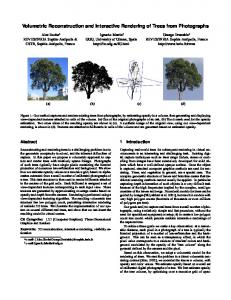
• All refinement ratios, i.e., all ratios of cell sizes between adjacent hierarchy levels, are integers (typically two or four). • Grid cells are never partially refined. An example of a 2D AMR hierarchy with three levels and a uniform refinement ratio of two is shown in Figure 1. Figure 2 shows the 3D grid structure of a real AMR data set. (a)

(b)

Figure 1: Three-level AMR hierarchy with a uniform refinement ratio of two. Grid boundaries are denoted by bold lines. All hierarchy levels consist of two grids. Note that finer grids can cross boundaries between coarser grids. (a) View of finest-resolution cells only. (b) “Exploded” view of AMR hierarchy. Shaded cells are “hidden” by finer-resolution grids. Though AMR methods are advantageous for the simulation of certain physical phenomena, they pose problems when one wants to visualize simulation results. Most existing visualization algorithms cannot handle AMR data directly, and the strategy used in the past was to resample AMR data onto a uniform grid (typically at the finest resolution present in a given AMR hierarchy). This approach does not work well, because the AMR grid structure – often interesting itself – is lost, and, due to the AMR data’s multiple resolution levels, resampled data tends to be too large to support efficient visualization. Considering a 3D AMR data set containing 16 levels of resolution (common in astrophysical simulations) with a uniform refinement ratio of two, a
3 resampled grid would consist of at least 215 cells.

• All grids are Cartesian. • Grids in the same hierarchy level, i.e., grids having the same cell size, do not overlap. ∗ Center for Image Processing and Integrated Computing (CIPIC), University of California, Davis † Fachbereich Informatik, Universit¨ at Kaiserslautern ‡ Visualization Group, Ernest Orlando Lawrence Berkeley National Laboratory

Figure 2: Argon Bubble data set. AMR hierarchy consisting of three levels, with refinement ratios of two and four, and 528 grids in total. Image shows AMR grid structure blended into volume rendering. It is therefore necessary to develop visualization algorithms that can handle AMR data directly and exploit the

structure of AMR data for visualization. AMR hierarchies are a collection of Cartesian grids, and efficient visualization techniques exist for those; and AMR hierarchies are inherently multiresolutional. Even though coarser grids may partially be overlaid by finer ones, the “hidden” cells still contain meaningful data, albeit at a lower resolution. Thus, it is possible to visualize low-resolution approximations of the complete AMR hierarchy by ignoring some of the finer levels. Due to the size of typical AMR data sets (gigabytes to terabytes) it is often not practical to move a data set to a user’s machine for interactive visualization. Therefore, an AMR visualization system should support remote rendering. In such a distributed system, the rendering takes place on the machine that generated and/or stores the data, and user interaction and display take place on the user’s machine. Remote rendering saves the cost of transmitting large amounts of data to a user’s machine, and enables the use of high-performance hardware located at a remote site. It is highly desirable that remote rendering is interactive, even if a user’s machine is connected to the rendering server via the Internet. We present an interactive volume visualization algorithm that reads an AMR data set in its native file format, splits the AMR hierarchy into a set of Cartesian grid patches on-the-fly, renders those patches using standard DVR algorithms, and composites the results into a final image. The algorithm can easily be adapted to several machine architectures by replacing the core rendering module, and it can be parallelized by scattering grid patches across several CPUs for independent rendering and gathering partial images during compositing. We have implemented (i) a single-CPU, hardware-assisted renderer for smaller data sets stored on a user’s desktop computer; (ii) remote, parallel, hardwareassisted renderers for clusters of PC-based graphics workstations or high-end multi-pipe graphics workstations; and (iii) a remote, massively parallel, software-only renderer for supercomputers. The “thin client” for remote rendering could be implemented as a web browser applet.

2

Related Work

DVR algorithms have been an active area of research for at least the last decade [5]. Many DVR algorithms are designed for Cartesian grids, and most can be used for the core rendering module in our visualization systems, e. g., ray casting [6], cell projection [7], shear-warp transform [8], and hardwareassisted texture-based volume rendering [10, 11, 12]. Some DVR algorithms suitable for unstructured grids, e. g., cell projection [7], its polygonal approximation [13], and incremental slicing [14], can also be applied to AMR hierarchies [15].

3

the first step, we split an AMR hierarchy into a set of non-overlapping Cartesian grid patches. This step is performed only once, on-the-fly, while loading an AMR data set’s grid structure, and does not involve resampling. This step typically requires only a fraction of a second. (2) Domain decomposition. For parallel rendering, the grid patches have to be distributed across processing nodes for rendering. Nodes have to load only those parts of an AMR data set that they are assigned to, allowing us to render large AMR data sets that do not fit into memory on a single processing node. We have investigated two different methods to perform load balancing during domain decomposition that do not require communication between processing nodes. (3) Back-to-front grid patch rendering. The grid patches assigned to a processing node are rendered using standard DVR algorithms. Our current softwareonly renderer uses a simple cell projection algorithm, whereas the hardware-assisted renderers employ the 3D texture mapping capabilites of high-end graphics workstations or current consumer-level graphics boards [10, 11, 12]. (4) Image compositing. For parallel rendering, the partial images generated independently by the processing nodes have to be composited into a single final image. Currently, we use a simple binary-tree based compositing algorithm. More advanced parallel compositing algorithms, e. g., binary swap [19], will be investigated in the future. The following sections describe these steps in more detail. Since Steps 2 and 4 only apply to the parallel rendering algorithm, and since they are closely related to each other, they are treated together in Section 3.3.

3.1

Grid Homogenization

For rendering, our algorithm splits an AMR data set into a set of non-overlapping grid patches. A grid patch is defined as a rectangular subgrid of a single grid in an AMR hierarchy. This definition implies that all cells in a grid patch are of identical size, and the grid patch’s data belongs to a single grid and is therefore stored in a single contiguous region of memory. These properties ensure that any grid patch can be rendered by standard DVR algorithms. The set of grid patches is constructed in such a way that it covers the entire domain of the AMR data set, and that it represents the finest resolution existing at any point. We call the process of tiling a data set’s domain with grid patches grid homogenization.

Volume Rendering AMR Data

We decided not to develop DVR techniques specific for AMR data, but instead to homogenize a given AMR data set such that it can be rendered with existing DVR algorithms for Cartesian grids. This strategy allows us to adapt our renderer to different machine architectures by merely replacing the core rendering module. We split the process of rendering AMR data into the following four steps:

Figure 3: Three overlapping grids from two different hierarchy levels split into grid patches. Boundaries between grids are denoted by bold lines; individual grid patches are denoted by different textures.

(1) Grid homogenization. Most DVR algorithms are optimized for Cartesian grids. Considering this fact, in

Grid homogenization is performed by overlaying a kdtree [17] onto the domain of an AMR data set, such that

each grid patch in the homogenized AMR data set is represented by one kd-tree leaf. Initially, the tree consists of a single leaf representing the entire domain. Grids from the AMR hierarchy are subsequently inserted one-by-one, in order of increasing resolution1 . Each grid to be inserted is implicitly split into a set of grid patches by existing interior kd-tree nodes while traversing the tree downwards, see Figure 4(a–b). When an interior node is completely contained inside one of those patches, it and its subtree are replaced by a leaf representing that patch. If, on the other hand, an existing kd-tree leaf is partially overlaid by a grid patch, that leaf is recursively split into a set of non-overlapped patches and a single overlaid patch. The latter is then replaced by the new higher-resolution grid patch, see Figure 4 (c). The complete kd-tree generated by homogenizing the AMR data set from Figure 1 is shown in Figure 5. (a)

(b)

(c)

one grid patch has been rendered as an RGB image with α-channel, it can be composited into the image representing all patches behind it by performing an “over” operation [16], either performed in software or in hardware as an α-blending operation. In the special case of a texture-mapping based hardware-assisted DVR algorithm [10, 11, 12], compositing can be performed implicitly by rendering all grid patches into the same frame buffer. The view-independent kd-tree generated during grid homogenization is also used to efficiently enumerate all grid patches in correct rendering order. An interior kd-tree node can be interpreted as a plane dividing the node’s domain into two regions, with one child node representing each region and no node in either subtree intersecting the dividing plane. This interpretation leads to a directed depth-first traversal scheme for the homogenizing kd-tree: At each internal node, the viewpoint is compared with the node’s dividing plane, and the subtree corresponding to the region “behind” the plane (as seen from the viewpoint) is traversed first; the other region is traversed second. Since the two regions are separated by the dividing plane, no grid patch rendered during the first traversal can occlude any grid patch rendered during the second traversal. By applying this step recursively we obtain a unique back-to-front ordering of all grid patches in the kd-tree. This approach leads to correct compositing, even if the viewpoint is inside the AMR data set’s domain. Note that the ordering algorithm is based solely on the viewpoint and is independent of viewing direction. The grid patch order imposed by traversing the kd-tree from Figure 5 is shown in Figure 6.

Figure 4: Inserting grid into kd-tree generated during grid homogenization. (a) Kd-tree structure before insertion of dashed grid. (b) Inserted grid split into patches after traversing existing tree. (c) New kd-tree generated by splitting partially overlaid leaves.

7

18

17

16 15

(a)

3

13

11

9

5

10

6

2 4

14 8

1

12

(b)

Figure 6: Grid patch order imposed by traversing the homogenizing kd-tree from Figure 5 in back-to-front order (viewpoint indicated by “×”). (c)

Figure 5: Homogenizing AMR data set from Figure 1. (a) Kd-tree after insertion of both level–0 grids. (b) Tree after insertion of both level–1 grids. (c) Final tree after insertion of both level–2 grids. Newly inserted grids are shaded.

Once the grid patches are ordered correctly, they are passed to the core rendering module individually. Our current implementation contains two different renderers: one is a standard cell-projection renderer [7] intended to be used on massively parallel supercomputers, the other one is a texture-mapping based, hardware-assisted renderer [10, 11, 12] for single or clustered PC-based, desktop graphics workstations using commodity graphics hardware (NVidia GeForce3) or high-end graphics workstations (SGI Onyx2 with multiple Infinite Reality2 pipes). 3.2.1

3.2

Back-to-front Grid Patch Rendering

The idea behind our approach is to render each of the grid patches generated during homogenization independently, using a standard DVR algorithm, and then to composite the individual results. The compositing step is especially simple if grid patches are rendered in back-to-front order [16]. If 1 Grids inside the same hierarchy level do not need to be inserted in any particular order.

Hardware-assisted Rendering

A typical 3D texture-mapping based volume renderer defines a 3D array of scalar data as a single intensity-only 3D texture and the accompanying transfer function as a color table mapping from intensity to (RGB, α) tuples. The renderer subsequently visualizes the volume by generating and rendering textured slices inside the data’s domain. Typically, slices are polygonal intersections between equidistant view-orthogonal planes and the data’s domain, see Figure 7. Slices are processed in back-to-front order, texture-mapped by generating appropriate texture coordinates for their vertices, and

rendered using α-blending, implicitly compositing them into the frame buffer. If the frame buffer provides sufficient precision for accurate α-blending, this sequence of operations is equivalent to numerically evaluating the volume rendering integral [5]. The effect of varying frame buffer precision on rendering results is shown in Figure 9. (a)

(b)

Figure 7: Generating view-orthogonal slices through a rectangular domain. (a) 2D example, with viewpoint (×) and view direction indicated in the lower-left corner. (b) Isometric view of 3D example, with viewing direction along the cube’s main diagonal. Note that slices change from triangles to hexagons and back to triangles. In the algorithm described by van Gelder and Kim in [11], slice polygons are generated by creating a stack of vieworthogonal rectangles whose projections contain the domain’s projection. Those rectangles are clipped against the domain using OpenGL’s clipping planes, and texture coordinates for their vertices are generated using OpenGL’s texture matrix. Yagel et al. [14] described a different approach to slice generation based on a 3D generalization of scan conversion. Their algorithm generates slices in software, by maintaining a list of active edges intersected by a current slice, and incrementing intersection points and (RGB, α) tuples as the current slice moves towards the viewpoint. To adapt this algorithm to texture-mapping based rendering, one has to iterate a current slice through a complete grid patch instead of a single cell, and has to increment texture coordinates along the active edges instead of color values. Unstructured grids cannot always be ordered in back-to-front order; therefore, the original slicing algorithm has to maintain an active cell list of all cells intersected by the current slicing plane, and it must increment all current slices in parallel. The adapted version does not need an active cell list, and only needs to slice one grid patch at a time. Grid patches can be ordered by traversing the homogenizing kd-tree and can be rendered individually. We chose the algorithm in [14] as it does not suffer from the inaccuracies inherent in vertex clipping and texture coordinate generation that sometimes mar OpenGL implementations. Our algorithm renders a volume by compositing multiple, independently rendered grid patches; therefore, it is important that the generated polygons and their texture coordinates match exactly across grid patch boundaries, see Figure 8(a). Doubly rendered or missing pixels along the boundaries would introduce highly visible artifacts. Using our algorithm, polygons always match up “pixel-accurately,” making the composited rendering indistinguishable from one generated from a single block. Since the main CPU mostly waits for OpenGL’s rasterization stage during slice rendering, the time needed to generate slices in software is hidden, leading to no observable perfomance penalty. Rendering grid patches of different cell sizes using textured slice polygons introduces two kinds of visual artifacts [18]. The first artifact stems from the limited precision of color representation in consumer-level graphics boards. Since grid patches containing higher-resolution data are ren-

dered using more slices, the opacity levels of the transfer function for those slices have to be reduced properly. If the reduced opacity values cannot be represented exactly, grid patches of different resolution levels will appear to have different “total opacities,” illustrated in Figure 9. The second kind of artifact is introduced by mismatching slice polygons across different-resolution grid patch boundaries, illustrated in Figure 8(b). The dotted lines parallel to the viewing direction denote a region where a higher-resolution slice polygon enters an image region rendered by two lower-resolution slices. This leads to a “staircasing” effect in total opacity along boundaries between grid patches of different resolutions. It turns out that the second kind of artifact is much less apparent than the first one; we could not detect it in our renderings. (a)

(b)

Figure 8: Rendering multiple grid patches of varying resolutions. (a) Slice polygons rendered for AMR data set from Figure 1: slice distance inside a grid patch is proportional to patch’s cell size. (b) Rendering artifact between two neighbouring patches belonging to different hierarchy levels.

(a)

(b)

Figure 9: Effect of limited-precision color representation on multiresolution rendering. (a) Image rendered on an NVidia GeForce3 graphics card with 8 bits of color precision. (b) Image rendered on an SGI Onyx2 with Infinite Reality2 graphics pipe and 12 bits of color precision, using identical data set and viewing parameters.

3.3

Domain Decomposition and Image Compositing

The major difficulty in parallelizing a volume rendering algorithm is designing a domain decomposition strategy, i. e., a strategy deciding how to assign parts of a data set to each processing node, and a compatible compositing strategy, i. e.,

a strategy deciding how to composite partial images. Available strategies have to be evaluated in terms of memory efficiency, load balancing and compositing complexity. “Perfect memory efficiency” is achieved when no data is stored by more than one node; “perfect load balancing” is achieved when all nodes require the same amount of time to render their assigned parts of the data. Compositing complexity is the time required to gather partial images from all nodes and composite them into a final image. Due to the irregular structure of AMR data, it is difficult to design a domain decomposition strategy that performs optimally in all three regards. We have investigated two different methods: cost range decomposition and domain block decomposition. Both methods are based on the viewindependent kd-tree generated during grid homogenization and are comparable in terms of compositing time, while the former favors load balancing and the latter favors memory efficiency. Both methods rely on the existance of an efficient means to estimate a grid patch’s rendering cost. Considering the two rendering algorithms we have implemented, and ignoring perspective foreshortening, the cost of rendering a grid patch is roughly proportional to the number of cells it contains, and to the projected size of each cell. The cell projection renderer has to process each cell individually and has to generate ray segments for each pixel in each cell’s projection. The texture-mapping based renderer has to upload all cell values into graphics card memory and has to composite all generated slice polygons into the frame buffer using α-blending. During grid homogenization, we store the rendering cost for each kd-tree node. The cost of a leaf is the estimated cost of rendering the grid patch it represents, and the cost of an interior node is the sum of costs of its two children. We describe our two decomposition strategies in detail in the following sections. 3.3.1

Cost-range Decomposition

This decomposition strategy is based on the observation that a back-to-front traversal of the homogenizing kd-tree imposes a unique view-dependent order on the kd-tree leaves. When representing each kd-tree leaf as an interval as wide as its estimated cost, and stacking those intervals next to each other in rendering order, one effectively splits the total cost interval into many different-sized pieces. To assign leaves to n rendering nodes for rendering, we split the total cost interval into n equal-sized sub-intervals, and assign those leaves that are at least half inside sub-interval i to rendering node i, see Figure 10(a). If the cost estimates are accurate, this strategy leads to perfect load balancing during rendering. The cost intervals are never really constructed; all decisions about traversing or skipping parts of the kd-tree are made during back-to-front traversal, without requiring additional communication between nodes. Image compositing is especially simple when using this strategy. Even though the domain regions assigned to each node are typically irregular in shape, no grid patch G rendered by node i can be occluded by any grid patch rendered by node i − 1, and G can never occlude any grid patch rendered by node i + 1, see Figure 10(b–c). This fact is due to ordering the grid patches in rendering order before assigning regions. In order to create a final image, it is sufficient to composite all partial images in order of (increasing) node index. We have implemented a binary tree compositing algorithm that requires dlog ne compositing rounds for n nodes. In each compositing round, a node either sends its image to

another node, receives an image and composites it into its own image (using either software or hardware), or is idle. (a) node 1

node 2

node 3

node 4

(b) 7

3

13 18

17

16

11

9

5

10

6

2 4

14

15

8

1

12

(c) 7

2

13 12

16

15 17

10

8

4

9

5

1 3

14 11

6

18

Figure 10: Cost-range decomposition for the example AMR data set from Figure 1. (a) Cost interval determined by back-to-front order from Figure 6; split into four equal-size regions. (b) Grid patch assignment for viewpoint (×) to the left of domain. (c) Different grid patch assignment for viewpoint (×) below domain (cost interval not shown). Cost-range decomposition achieves good load balancing in practice, see Section 6. Its main drawback is poor memory efficiency. Even when an AMR data set is rendered for the first time, the view-dependent region assignment might assign grid patches belonging to the same grid to multiple rendering nodes, forcing each of those nodes to load all data associated with the grid. When changing the viewpoint during interactive rendering, grid patches change assignment due to changes in rendering order, see Figure 10(b–c), forcing the algorithm to replicate data between more nodes. Though reloading happens incrementally, and does typically not impact interactive rendering, after several viewpoint changes the entire data set might be replicated at every node. 3.3.2

Domain Block Decomposition

This decomposition strategy is based on the observation that any intermediate stage in a breadth-first traversal of a homogenizing kd-tree can be rendered in back-to-front order. If the entire kd-tree is split into n subtrees, and each subtree is assigned to one of the n rendering nodes, there exists a node ordering such that the same compositing strategy used in cost-range decomposition can be used to composite the partial images associated with each subtree. We split a homogenizing kd-tree into roughly equal-cost subtrees using the following heuristic: Initially, we create a priority queue containing only the root node. While the number of nodes in the queue is smaller than the number of rendering nodes, the most expensive node is removed from the queue, and its two children are inserted. This domain decomposition is view-independent and therefore does not require loading of data during interactive rendering. There can still be data replication due to grid patches belonging to the same grid being assigned to multiple subtrees, but in practice memory efficiency is good. Compositing time is almost as good as in cost-range de-

composition: After dlog ne compositing rounds, the node assigned to the “farthest” subtree will have created the final image. In cost-range decomposition, this node is always node 0, the master node. In domain block decomposition, however, the final image might have to be sent to the master node in an additional step. The major drawback of domain block decomposition is that good load balancing can only be achieved if the homogenizing kd-tree is well-balanced. As mentioned in Section 3.1, grids inside the same hierarchy level can be inserted into the kd-tree in any order; this freedom can be exploited to construct better-balanced trees.

4

Remote Rendering

We have implemented distributed AMR volume renderers based on the algorithms described above, to support rendering of AMR data sets that are too large to fit into desktop computer memory, and to support using high-end graphics hardware available at supercomputing centers. Unlike the Visapult distributed rendering system [20], which uses client-side compositing to guarantee limited interactivity in the presence of network problems, our system follows a “thin client” approach, i. e., data is only stored at a remote rendering server, and all rendering and compositing occurs remotely. The client only receives final, composited RGB images from the server, and the client supports a user interface to select rendering parameters and interactively change viewpoints. The absence of any 3D rendering requirements allows one to implement a version of the client in a completely platformindependent way, e. g., as a Java applet. The drawback of the thin client approach, requiring a full round-trip and transmission of a final image between client and server for each update during interactive rendering, is offset by allowing onthe-fly JPEG compression of transient images. Experiments have demonstrated that the thin client approach supports interactive visualization of large AMR data sets at several frames per second, even under the latency and bandwidth constraints of a consumer-level DSL Internet connection.

5

(a)

(b)

(c)

Ensuring Interactivity

To ensure interactive frame rates while rendering arbitrarily large data sets, our system exploits the multiresolution structure of AMR data. The simplest way to render lowerresolution approximations is to ignore some of the more refined levels during grid homogenization. Since coarserresolution cells that are overlaid by finer-resolution cells contain valid data, ignoring increasing numbers of finerresolution levels will gracefully decrease image quality and rendering time, see Figure 11. More advanced strategies that take viewing parameters into account to determine if, and at which resolution level, to render parts of a data set could be developed as well. In our current implementation, a user can adjust two settings: the resolution level for rendering still images and the resolution level for rendering transient images during interactive viewpoint changes. Another option is to reduce image resolution during interaction, and to enlarge the resulting image using OpenGL’s pixel zoom feature. Combining both techniques, we have been able to achieve interactive rendering rates of at least five frames per second for all data sets we have used to date.

Figure 11: Rendering AMR data set at multiple levels of resolution. (a) Base level only, consisting of three grids and 81,920 cells. (b) Levels zero and one, consisting of 26 grids and 291,206 cells. (c) All three levels, consisting of 541 grids and 6,788,900 cells.

Data

# of

Set

Levels

Configurations Single PC

SGI Onyx2

PC Cluster

Argon

1

0.00

0.00

0.00

0.1

0.1

0.1

0.1

0.1

0.1

Bubble

2

0.03

0.02

0.02

0.1

0.1

0.1

0.1

0.1

0.1

3

0.66

0.12

0.10

0.1

0.1

0.1

0.1

0.1

0.1

1

2.90

0.30

0.30

0.1

0.1

0.1

0.1

0.1

0.1

X-Ray

2

0.1

0.1

0.1

0.1

0.1

0.1

0.1

0.1

0.1

Cluster

5

0.1

0.1

0.1

0.1

0.1

0.1

0.1

0.1

0.1

10

0.1

0.1

0.1

0.1

0.1

0.1

0.1

0.1

0.1

Table 1: Performance measurements for two example data sets (Argon Bubble and X-Ray Cluster) for three rendering configurations. Under each configuration, first columns list times needed to render initial image (including data load); second columns list times needed to render static image; third columns list times needed to render transient image. (All measurements in seconds)

6

Examples and Results

We have timed our algorithms for two example data sets (one small, one very large) on several rendering environments. The resulting rendering times per frame are listed in Table 1. Data Set 1 (Argon Bubble). This time-varying data set, provided by The Center for Computational Sciences and Engineering at the Lawrence Berkeley National Laboratory 2 , consists of 501 timesteps. Each timestep contains three hierarchy levels, using refinement ratios of two and four, and between 200 and 900 grids in total (varying with timestep). The domain size is 256 × 256 × 640 finest-level cells; actual data size is between 2.5 and 9.5 million cells. Images of several timesteps of this data set are shown in Figures 2, 9 and 11. Data Set 2 (X-Ray Cluster). This data set, provided by Mike Norman of SDSC and Greg Bryan of Princeton contains ten hierarchy levels, using a uniform refinement ratio of two, and 34,494 grids in total. The domain size is 131, 072 × 131, 072 × 131, 072 finest-level cells; actual data size is 53,041,374 cells. Desktop Graphics Workstation. The computer used was an off-the-shelf PC (Intel Pentium 4, 1.8 GHz, 512 MB RAM, AGP 4×, NVidia GeForce3, 64 MB, 60 GB EIDE HD). The rendered data sets were stored on the local harddrive. High-end Graphics Workstation. The computer used was an 8-processor SGI Onyx2 visualization server with two Infinite Reality2 graphics pipes (two RM7 on pipe 0, one RM9 on pipe 1, 64 MB texture memory each). The rendered data sets were stored on a high-performance local disk array. Cluster of PC-based Graphics Workstations. The computers used were off-the-shelf PCs (Intel Pentium 4, 2.0 GHz, 512 MB RAM, AGP 4×, NVidia GeForce3 Ti 200, 64 MB, 60 GB EIDE HD) connected via 100 Mbit/s Ethernet. The rendered data sets were stored on the master’s local harddrive and accessed by the slaves via NFS. 2 See http://seesar.lbl.gov/ccse, http://seesar.lbl.gov/ccse/Research/Hyperbolic.

7

Conclusions and Future Work

We have presented an algorithm that renders AMR data sets by splitting them into homogenuous grid patches on-the-fly while loading a data set’s grid structure. The algorithm subsequently renders grid patches independently using standard DVR algorithms. By exploiting the multiresolution structure of AMR data, hardware-assisted implementations of our algorithm can render extremely large data sets at interactive rates, even when data is stored and rendered remotely. Using a thin client approach that allows one to implement a rendering client as a Java applet, the remote rendering system can be integrated into distributed environments for scientific computing. Our current implementation could benefit from improvements in two main areas: First, it will be worthwile investigating better strategies for domain decomposition and image compositing for parallel rendering; and second, it will be advantageous to replace the existing core rendering modules with higher-quality renderers. Recent advances in consumer-level graphics hardware enable many desirable improvements, including hardware-assisted illumination. Acknowledgments. This work was supported primarily by the Director, Office of Science, Office of Advanced Scientific Computing Research, Mathematical, Information, and Computational Sciences Division, U.S. Department of Energy under Contract No. DE–AC03–76SF00098. It was also supported by the National Science Foundation under contract ACI 9624034 (CAREER Award), through the Large Scientific and Software Data Set Visualization (LSSDSV) program under contract ACI 9982251, and through the National Partnership for Advanced Computational Infrastructure (NPACI); the Office of Naval Research under contract N00014–97–1–0222; the Army Research Office under contract ARO 36598–MA–RIP; the NASA Ames Research Center through an NRA award under contract NAG2–1216; and the Lawrence Livermore National Laboratory under ASCI ASAP Level–2 Memorandum Agreement B347878 and under Memorandum Agreement B503159. We also acknowledge the support of ALSTOM Schilling Robotics and SGI. We thank the members of the Visualization Group at the Lawrence Berkeley National Laboratory and the members of the Visualization and Graphics Research Group at the Center for Image Processing and Integrated Computing (CIPIC) at the University of California, Davis.

References [1] Berger, M. J., and Oliger, J., Adaptive Mesh Refinement for Hyperbolic Partial Differential Equations, Journal of Computational Physics 53 (1984), pp. 482–512 [2] Berger, M. J., and Colella, P., Local Adaptive Mesh Refinement for Shock Hydrodynamics, Journal of Computational Physics 82 (1989), pp. 64–84 [3] Pember, R. B., Bell, J. B., Colella, P., Crutchfield, W. Y., and Welcome, M. L., An Adaptive Cartesian Grid Method for Unsteady Compressible Flow in Irregular Regions, Journal of Computational Physics 120 (1995), pp. 278–304 [4] Aftosmis, M. J., Berger, M. J., and Melton, J. E., Adaptive Cartesian Mesh Generation, in: Thompson, J. F., Soni, B. K., and Weatherill, N. P., eds., Handbook of Grid Generation (1999), CRC Press, Boca Raton, Florida, pp. 22-1–22-26 [5] Drebin, R. A., Carpenter, L. and Hanrahan, P., Volume Rendering, Computer Graphics 22(4) (Proc. SIGGRAPH ’88) (1988), pp. 65–74 [6] Levoy, M., Display of Surfaces from Volume Data, IEEE Computer Graphics and Applications 8(3) (1988), pp. 29–37 [7] Max, N. L., Hanrahan, P. and Crawfis, R., Area and Volume Coherence for Efficient Visualization of 3D Scalar Functions, Computer Graphics 24(5) (Proc. SIGGRAPH ’90) (1990), pp. 27–33 [8] Lacroute, P., and Levoy, M., Fast Volume Rendering Using a Shear-Warp Factorization of the Viewing Transformation, Computer Graphics 28(4) (Proc. SIGGRAPH ‘94) (1994), pp. 451–458 [9] Westover, L., Footprint Evaluation for Volume Rendering, Computer Graphics 24(4) (Proc. SIGGRAPH ’90) (1990), pp. 367–376 [10] Cabral, B., Cam, N. and Foran, J., Accelerated Volume Rendering and Tomographic Reconstruction Using Texture Mapping Hardware, Proc. 1994 ACM Symposium on Volume Visualization (1994), ACM Press, New York, New York, pp. 91–98 [11] Van Gelder, A. and Kim, K., Direct Volume Rendering with Shading via Three-Dimensional Textures, Proc. 1996 Symposium on Volume Visualization (1996), IEEE Computer Society Press, Los Alamitos, California, pp. 23–ff. [12] Rezk-Salama, C., Engel, K., Bauer, M., Greiner, G. and Ertl, T., Interactive Volume Rendering on Standard PC Graphics Hardware Using MultiTextures and Multi-Stage Rasterization, Proc. 2000 SIGGRAPH/EUROGRAPHICS Workshop on Graphics Hardware (2000), held in Interlaken, Switzerland, ACM Press, New York, New York, pp. 109–118 [13] Shirley, P. and Tuchman, A., A Polygonal Approximation to Direct Scalar Volume Rendering, Computer Graphics 24(5) (San Diego Workshop on Volume Visualization) (1990), pp. 63–70

[14] Yagel, R., Reed, D. M., Law, A., Shih, P.-W. and Shareef, N., Hardware Assisted Volume Rendering of Unstructured Grids by Incremental Slicing, Proc. 1996 Symposium on Volume Visualization (1996), IEEE Computer Society Press, Los Alamitos, California, pp. 55–ff. [15] Weber, G. H., Kreylos, O., Ligocki, T. J., Shalf, J. M., Hagen, H., Hamann, B., Joy, K. I. and Ma, K.-L., HighQuality Volume Rendering of Adaptive Mesh Refinement Data, in: Ertl. T., Girod, B., Greiner, G., Niemann, H. and Seidel, H.-P., eds., Vision, Modeling and Visualization 2001 (2001), IOS Press, Amsterdam, The Netherlands, pp. 121–128 [16] Porter, T. and Duff, T., Compositing Digital Images, Computer Graphics 18(3) (Proc. SIGGRAPH ‘84) (1984), pp. 253–259 [17] Samet, H., The Design and Analysis of Spatial Data Structures (1999), Addison-Wesley Publishing Company, Inc., Reading, Massachusetts [18] LaMar, E. C., Hamann, B. and Joy, K. I., Multiresolution Techniques for Interactive Texture-Based Volume Visualization, in: Ebert, D., Gross, M. H. and Hamann, B., eds., Proc. Visualization ’99 (1999), IEEE Society Press, Los Alamitos, California, pp. 355–361, 543 [19] Ma, K.-L., Painter, J. S., Hansen, C. D. and Krogh, M. F., A Data Distributed, Parallel Algorithm for RayTraced Volume Rendering, Proc. 1993 Symposium on Parallel Rendering (1993), ACM Press, New York, New York, pp. 15–22 [20] Bethel, E. W., et. al., Using High-Speed WANs and Network Data Caches to Enable Remote and Distributed Visualization, in: Proc. IEEE SC2000, The SCxy Conference Series, Dallas, Texas, November 2000