Remote sensing inputs and a GIS interface for ... - Hydrologie.org

Remote Sensing and Hydrology 2000 (Proceedings of a s y m p o s i u m field at Santa Fe, N e w Mexico, U S A , April 2000). I A H S Publ. no. 267, 2 0 0 1 .

421

Remote sensing inputs and a GIS interface for distributed hydrological modelling

G R E G S. CROSBY, CHRISTOPHER M. U. N E A L E Department of Biological and Irrigation Blvd. Logan, Utah 84322-4105, USA

Engineering,

Utah State

University,

4105

University

e-mail: [email protected]

M A R K SEYFRIED USDA-ARS,

Northwest

Watershed

Research

Center,

Boise,

Idaho

83712-7716,

USA

DAVID T A R B O T O N Department of Civil and Environmental Blvd. Logan, Utah 84322-4110, USA

Engineering,

Utah State

University,

4110

University

Abstract High resolution aerial (0.3-3.0 m) multispectral imagery was acquired over several sub-basins of the Reynolds Creek Experimental Watershed (RCEW) in 1996 to provide various spatial resolution imagery for the development of vegetation-related GIS layers (LAI, percent cover, vegetation type, canopy height, root depth, etc.). Thematic Mapper (TM) imagery (30 m) was also collected for the entire RCEW. The imagery will provide data to a remote sensing input driven hydrological model. This paper concentrates on the development of the GIS layers in the ArcView environment to be used with the distributed hydrological model. Key

words

GIS; LAI; multispectral imagery; remote sensing; N D V I ; Reynolds Creek

Experimental Watershed; RVl; SAVI; semiarid watershed

INTRODUCTION Data collection over large areas has not been possible, making it difficult to apply models over large watersheds. Remotely sensed imagery offers a method of collecting data across various spatial scales to parameterize inputs to a distributed model and provide verification of model outputs (Artan, 1996). The objectives of this paper are: (a) to develop a relationship between high spatial resolution (0.3 m) airborne multispectral digital video imagery and ground based canopy leaf area index (LAI) and percent cover measurements for various modelling scales, and (b) to demonstrate the creation of model input data in a GIS environment that may be accessed by a distributed hydrological model.

BACKGROUND Site description The research was conducted at the Reynolds Creek Experimental Watershed (RCEW) in the Owyhee Mountains of southwestern Idaho, USA. Reynolds Creek is a semiarid

422

Greg S. Crosby et al.

watershed where the hydrological processes are highly variable and dependent on precipitation (primarily snow) and évapotranspiration. The watershed has an area of 23 400 ha and is primarily used for grazing. There are areas of junipers, Douglas fir and aspen in the upper elevations and rangeland species are found throughout. The watershed has an average of 250 m m of annual precipitation at its lower elevations and over 1000 m m at the highest elevations with 7 5 % falling as snow. One of the advantages of this research watershed is the monitored sub-basins of varying sizes that are located within the watershed at various elevations (1098— 2254 m). Nancy's Gulch is the most northern sub-basin being studied and has the lowest elevation and the least slope. The basin consists primarily of small sagebrush, perennial grasses and other small vegetation. The Lower Sheep Creek sub-basin is a 13.25 ha sub-basin located at 1622 m comprised entirely of sagebrush rangeland. Whiskey Hill is located in the higher elevations and consists of a big mountain sagebrush community with mixed shrubs and perennial grasses; however, some junipers and dry meadow site areas are present. Reynolds Mountain (40.47 ha) is located at an average elevation of 2073 m, predominantly covered with rangeland vegetation but scrub aspen, willow, and Douglas fir are also present. Tollgate is a 5444 ha watershed that encompasses the southern end of the Reynolds Creek experimental watershed.

Methodology Multispectral videography The second generation Utah State University (USU) airborne multispectral videography system (Neale, 1991; Neale & Crowther, 1994; Neale et al, 1997) was used to acquire high-resolution imagery (0.3, 0.6, 0.9 m) over the vegetation transects within each sub-basin throughout the season. Due to the varying topography, the flight altitudes were planned based on the average elevation of the sub-basin being flown. The methodology described by Crowther (1992) and Neale & Crowther (1994) for the first generation U S U system was used to reduce brightness errors with a vignetting correction. An Exotech radiometer was calibrated against the video cameras to develop a radiometric correction (Neale & Crowther, 1994). Aircraft motion effects (band interlacing) were removed using programs developed at the U S U Remote Sensing Services Laboratory, described by Neale et al. (1994). During each remote sensing flight, an Exotech radiometer with Thematic Mapper bands T M I - 4 was set up at the Nancy's Gulch sub-basin to acquire incoming irradiance over a calibrated barium sulphate panel with known bi-directional properties. Ground data The US Agricultural Research Service (ARS) in Boise, Idaho collected the vegetation cover and LAI field data using the point frame method (Canfield, 1941). Vegetation plots set up within each sub-basin were considered representative of the surrounding watershed. The plots consisted of five transects 1.2 m apart and 30 m long. White panels were set up at the four corners of this plot so that it could be readily observed in the multispectral imagery. The point frame (consisting of 20 rods with points) was moved along each transect. Only green vegetation hits were noted during field sampling. The locations were 1, 4, 12, 16, 24 and 28 m from the

Remote sensing inputs and a GIS interface for distributed hydrological

423

modelling

end, coinciding with frame numbers 1, 2, 4, 5, 7 and 8 respectively along a transect. The vegetation data were always collected close to the date of the image acquisition flights. Table 1 summarizes the dates for each flight and the vegetation data collected. Table 1 Data collection dates, 1996 (Julian day-of-year).

Nancy's Gulch Lower Sheep Whiskey Hill Reynolds Mountain

Ground

Airborne

Ground

Airborne

Ground

Airborne

152 155 151-152

158 158 158 158

215 215 218 218

215 215 215 215

247 247 247 247

242 242 242 242

ANALYSIS Ground data Percent cover was evaluated at each frame location by noting if at least one green hit occurred at a pin. The green hits (maximum of 20) were divided by 20 to estimate the area of land that was covered by green vegetation. The LAI was calculated by dividing the total number of green hits at a frame location by the total number of points within a frame (20).

Multispectral imagery Images were selected for analysis by observing which image had the vegetation plot located within the centre of the image. A registered 3-band image was produced. The resulting 3-band image was then calibrated to reflectance using the following equation:

_ K g,r,NiR DN

x

calibration^)/(voltageconv

_

-"•pixel

2629

)]xpanelref

v X

,

3630

(1)

panet ^3629 where i? j i is the reflectance of an individual pixel in an image, DN is the digital number of the green, red or NIR pixel, calibration is the linear relationship between DN and radiometer radiances (no. 3629) (W n f ) , voltageconv is voltage conversion for aircraft radiometer no. 3629 (W m" V" ), panelref is the bi-directional reflectance for the barium sulphate panel based on the sun's zenith angle, panel is the panel radiometer voltage readings, and v 3 o / v 6 2 9 is the cross-calibration of the radiometers over the panel A GPS time stamp on each image was used to correlate an image with the panel irradiance readings that were continuously being taken in the field. Panel measurements were averaged every minute so an interpolation was done between the two time measurements closest to the image. A normalized difference vegetation index [NDVI = (NIR + red)/(NIR - red)] image was calculated. The 3-band reflectance imagery was rectified to an imaginary grid that was based on the orientation of the ground vegetation transects. Plot no. 1 therefore contained the average ground data for the five Frame #1 sites for each transect 1-5. The means were compared with the corresponding ground data. 36i0

P

Xe

2

2

36

1

3

424

Greg S. Crosby et al.

The lower resolution (3 m) imagery was rectified to digital orthophotquads and the higher resolution imagery was rectified sequentially in turn down to the 0.3 m resolution imagery to match the data geographically. Contour and soil maps of the watersheds were digitized for creating the layers for the GIS. Vegetation type data were verified in the field with imagery in hand to aid in the supervised classification of the imagery and obtaining a vegetation layer. All of the image data have been converted into a grid file to be incorporated more easily into hydrological models. By using general information about the different vegetation types, tables were constructed to provide additional attributes such as plant height and root depth. Figure 1 presents a sample of some of the layers that are present in the GIS. The entire river network for the R C E W is shown with some of the sub-basins of interest. The 3-band mosaic of Reynolds Mountain is presented with the overlying river vector layer in the upper right; in the lower right, part of the vegetation layer table is presented for Upper Sheep Creek.

Fig. 1 GIS layers for Reynolds Creek Experiment Station.

RESULTS Table 2 shows N D V I data obtained from the calibrated imagery and ground data. A second order polynomial was used to fit a curve since increasing orders only provided

Remote sensing inputs and a GIS interface for distributed hydrological modelling

425

Table 2 Field data and imagery statistics for Whiskey Hill (June and August). Ground data day (multispectral).

Frame

Day 151 Hits Total hits

% cover

LAI

NDVI

Day 247: Hits Total hits

% cover

LAI

NDVI

1 2 4 5 7 8

69 78 83 65 75 67

117 160 170 130 152 119

0.69 0.78 0.83 0.65 0.75 0.67

1.17 1.6 1.7 1.3 1.52 1.19

0.341 0.39 0.406 0.362 0.369 0.348

28 32 43 22 40 16

44 44 64 34 69 20

0.28 0.32 0.43 0.22 0.4 0.16

0.44 0.44 0.64 0.34 0.69 0.2

0.201 0.259 0.197 0.143 0.235 0.136

Total

437

848

181

275

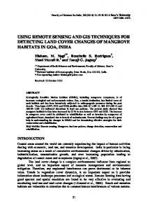
a small change in the R M S and did not follow the trend of the data but rather attempted more to follow the individual points. There was a strong relationship between the N D V I and ground biophysical data (percent cover and LAI) that were collected as indicated by the high R (Figs 2 and 3). It would have been helpful to have more heavily vegetated areas to improve the relation­ ships. Unfortunately, the Reynolds Mountain site did not yield expected higher LAI and percent cover data. July imagery was not included in the relationship as the presence of clouds on that flight date has posed some problems that are still unresolved. 2

2

y= 10.112x -0.8872x +0.1788 R = 0.8449 2

0

0.05

0.1

0.15

0.2

0.25

0.3

0.35

0.4

NDVI Fig. 2 NDVI vs LAI relationship. 2

y = 2.9976X + 0.5372x + 0.0805 2

R = 0.8365

NDVI Fig. 3 NDVI vs percent cover relationship.

0.45

Greg S. Crosby et al.

426

The Arc View GIS database and interface allows for hydrological model input data and visualization of model results. The vegetation classification was used to develop a distribution of vegetation characteristics such as plant height and root depth that can further be characterized by location, altitude, etc. The database makes it easier to continue to add to the project to better represent the basins and influence/test the model outputs. Imagery acquired at different spatial resolutions will be used along with this high-resolution layer, to study the effects of scaling-up some of the parameters to larger sub-basins. Views have been constructed within the project which will allow one to see the research that was done and observe the data that was collected.

A c k n o w l e d g e m e n t s NSF-EPA Grant R824784 has funded this research. We greatly appreciate the assistance of Mark Murdock in collecting the field data.

REFERENCES Artan, G. (1996) A spatially distributed energy flux model based on r e m o t e l y sensed and p o i n t - m e a s u r e d

data.

Dissertation, Utah State University, Utah, U S A . Canfield, R. H. (1941) Application of the Line Interception Method in s a m p l i n g range vegetation. J. For. 3 9 , 3 8 8 - 3 9 4 . Crowther, B . (1992) Radiometric calibration of multispectral video imagery. T h e s i s , Utah State University, L o g a n , Utah, USA. Neale, C. M. U. (1991) An airborne multispectral video/radiometer r e m o t e sensing system for agricultural and environmental monitoring. Paper presented at the A S A E S y m p . on A u t o m a t e d Agriculture for the 21st Century (Chicago, Illinois, U S A ) . N e a l e , C. M . U. & Crowther, B . G. (1994) A n airborne multispectral d e v e l o p m e n t and calibration. Remote

Sens. Environ.

video/radiometer r e m o t e sensing system:

49, 187-194.

N e a l e , C. M . U. et al. ( 1 9 9 7 ) Classification and m a p p i n g of riparian systems using airborne multispectral videography. Restoration

Ecology

5(4S), 1 0 3 - 1 1 2 .

Tarboton, D . G., Neale, C. M., Cooley, U. K., Flerchinger, G., Hanson, C , Seyfried, M. & Slaughter, C. W. (1994) Scaling up Spatially Hydrologie M o d e l s of Semi-Arid W a t e r s h e d s . Proposal, Logan, Utah, U S A .