IMAGE INTERPOLATION WITH DIRECTIONLETS Vladan ... - CiteSeerX

IMAGE INTERPOLATION WITH DIRECTIONLETS Vladan Velisavljevi´c

Raphael Coquoz

Deutsche Telekom Laboratories Berlin, Germany

Ecole Polytechnique F´ed´erale de Lausanne Lausanne, Switzerland

ABSTRACT We present a novel directionally adaptive image interpolation based on a multiple-direction wavelet transform, called directionlets. The algorithm uses directionlets to efficiently capture directional features and to extract edge information along different directions from the low-resolution image. Then, the high-resolution image is generated using this information to preserve sharpness of details. Our interpolation algorithm outperforms the state-of-the-art methods in terms of both numeric and visual quality of the interpolated image. Index Terms— Interpolation, directional, directionlet, locally adaptive, wavelet transforms.

(a)

(b)

(c)

(d)

1. INTRODUCTION Image interpolation commonly refers to generating missing image pixels from the available image information, which is often required in magnification. The task of magnification is an essential part of software zooming, focusing regions of interest or printer drivers. The main challenge is to preserve sharpness of images after resolution enhancement. The traditional magnification approaches based on bicubic or spline interpolation [1] are used because of fast computation, easy implementation and no a priori knowledge assumption. However, these methods generate blurred high-resolution (HR) images from their low-resolution (LR) counterparts. Our goal in this paper is to propose a method that reduces this blurring effect at HR. Several recent methods improve the visual quality of the interpolated images by exploiting the correlation among image pixels and modeling it using the Markov random field either in the wavelet [2, 3] or in the pixel domain [4]. Furthermore, in [4], Li and Nguyen characterize pixels as edge and non-edge and apply different interpolation algorithms to them. Edge-adaptivity and geometric regularity are also exploited in [5] and [6]. In the latter, the edge direction is extracted from the LR covariance matrices and is used to estimate their HR counterparts. However, the computation of the covariance matrices is limited only to the first four neighbor pixels. As a result, the reconstructed edges in the interpolated HR image are still blurred when compared to the edges in the original image. Another adaptive interpolation method has been proposed in [7]. This method makes use of the multiscale two-dimensional (2-D) wavelet transform (WT) to capture and characterize edges, which induce peaks in the wavelet subbands. The characterization involves estimation of location, magnitude and evolution of the corresponding peaks across wavelet scales determined by the local Lipschitz regularity of edges [8, 9]. This information is used to estimate the corresponding wavelet subbands in the HR multiscale decomposition and to generate the HR image by applying the inverse 2-D WT. The preserved characterization of edges at HR allows for sharpness

Fig. 1. A detail of the image Baboon is interpolated using three methods: traditional bicubic, locally adaptive wavelet-based and directionally adaptive interpolation based on directionlets. (a) The original HR image. (b) Bicubic interpolation with blurred details. (c) Wavelet-based interpolation is better, but it fails to capture efficiently directional features. (d) Our method based on directionlets outperforms the previous ones providing both higher numeric and visual quality and sharper edges in the interpolated images.

and a good visual quality of the reconstructed images. However, notice that the implemented WT is a separable transform constructed only along the horizontal and vertical directions [8]. Thus, it fails to characterize efficiently edges along different directions. Recently, the 2-D WT built along multiple directions (directionlets) has been proved [10, 11] to provide sparse representation of images and to improve the performance of wavelet-based image compression methods. This achievement motivates us to use directionlets to improve the characterization of edges in images along different directions necessary for the interpolation method in [7]. In our novel interpolation method, directionlets are constructed adaptively so that the chosen directions are maximally aligned with locally dominant directions across image. Because of the alignment, the transform

HR xo

LR 3-Band 2-D WT

LP

HR Extrapolation

HP

x

Bicubic

Iterative POCS

HP

Inverse 3-Band 2-D WT

xo est

LP

Fig. 2. Block diagram of the interpolation algorithm proposed in [7].

generates a sparser representation with a reduced energy in the highpass wavelet subbands allowing for a more robust estimation of the edge characteristics. The interpolated images achieve better numeric and visual quality than the images obtained by both the bicubic and the previous wavelet-based methods, as shown in Fig. 1. The outline of the paper is as follows. We review the interpolation method proposed by Chang et al. [7] and the basic properties of directionlets in Section 2. In Section 3, we present our interpolation method, where we first explain how to determine locally dominant directions and then we give the details of the algorithm. We show and compare interpolated images to the previous results in Section 4 and, finally, we conclude in Section 5. 2. REVIEW OF BACKGROUND WORK Here, because of lack of space, we give only a short review of the basic concepts of the interpolation algorithm in [7] and the construction of directionlets [10]. 2.1. Locally adaptive wavelet-based interpolation This algorithm is based on the assumption that the LR version is obtained from the HR original image as a low-pass output of the 3band 2-D WT, which is also used in [8]. The main idea is to estimate the corresponding missing HR low-pass and two high-pass subbands from the available LR image so that the inverse 3-band 2-D WT applied to these subbands provides a reconstructed HR image with preserved sharpness (see Fig. 2). The process of estimation of the 3 wavelet subbands consists of two phases: (a) initial estimate and (b) iterative projections onto convex sets (POCS). In the first phase, the initial estimates of all the 3 subbands at HR are computed. The low-pass subband is simply obtained by the bicubic interpolation of the LR image. However, since the high-pass subbands play an important role in obtaining sharp reconstructed image, they are generated using a more sophisticated method. First, a multiscale 3-band 2-D WT is applied to the LR image with 3 levels of decomposition. Then, extrema of the magnitudes of the wavelet coefficients are located in each row and column of the high-pass subbands to determine the position of sharp variation points (SVP). The extrema of the magnitudes at different scales j = 1, . . . , J related to a single SVP indexed by m follow the scaling relation [8] |W (j) f (xm )| = Km 2jαm , (1) where Km and αm are scaling constant and local Lipschitz regularity factor assigned to the mth SVP, respectively. These two parameters are estimated from the determined extrema in the wavelet subbands by linear regression and they are used to extrapolate the corresponding coefficient values in the HR high-pass subbands. The other high-pass coefficients that do not correspond to any SVP are filled by a simple linear interpolation along rows and columns. In the second phase, the estimated wavelet subbands are iteratively projected onto 3 convex sets determined by the following properties: (a) the 3 wavelet subbands must belong to the subspace of the wavelet transform, (b) the subsampled low-pass subband must

MΛ =

1 1 –1 1

s0 = 0 0 s1 = 0 1

M Λ′ =

2 2 –1 1

Fig. 3. An example of construction of directionlets based on integer lattices for pair of directions (45◦ , −45◦ ).

be consistent with the LR image and (c) the high-pass subbands must be consistent with the extracted SVP information. The final estimation of the wavelet subbands is transformed back to the original domain using the corresponding inverse 3-band 2-D WT to obtain the interpolated HR image. 2.2. Directionlets Directionlets are constructed as basis functions of the skewed anisotropic wavelet transforms [10]. These transforms make use of integer lattices to apply the scaling and wavelet filtering operations along a pair of directions, not necessarily horizontal or vertical. The basic operations are purely one-dimensional (1-D) and, thus, directionlets retain separability and simplicity of the standard 2-D WT. Notice that, even though the originally proposed transform in [10] is critically sampled (the filtering operations are followed by subsampling), here we use an oversampled version allowing for shift-invariance and making the extraction of edge information more robust. Fig. 3 shows an example of the construction of directionlets for pair of directions along (45◦ , −45◦ ). 3. DIRECTIONALLY ADAPTIVE INTERPOLATION The restriction of having only two directions in the construction of directionlets implies a need for spatial segmentation of image and adaptation of the transform directions in each segment. The assigned pairs of transform directions to each segment across the image domain form a directional map. The computation of such a map is explained in the sequel. 3.1. Directional map Image is first divided into spatial segments of the size 16 × 16 pixels.1 Directionlets are then applied in each segment along each pair of directions from the set D = {(0◦ , 90◦ ), (0◦ , 45◦ ), (0◦ , −45◦ ), (90◦ , 45◦ ), (90◦ , −45◦ )} using the biorthogonal ”9-7” 1-D filterbank [12]. Notice that the corresponding lattices for these pairs of directions do not divide the cubic lattice into more cosets, as explained in [10] in detail. To avoid a blocking effect in the transform caused by many small segments, the pixels from the neighbor segments are used for filtering across the segment borders. The best pair of directions d∗n ∈ D is chosen for each segment 1 Different

sizes do not influence significantly the final results.

(a)

WT, directionlets produce three high-pass subbands per scale denoted as HL, LH and HH according to the order of the low-pass and high-pass filtering in the two transform steps. In case of the subbands HL and LH, the search for SVP and the extraction of the SVP parameters are performed along the first and second transform directions, respectively (instead of the horizontal and vertical directions in the previous method), whereas, in case of the subband HH, this process is applied along any of the two directions. Owing to the properties of the applied transform, the extrema of the magnitudes of the di(j) rectionlets coefficients |WHL,LH,HH f (xm )| at scales j = 1, . . . , J follow the scaling relation [9]

(b)

(j)

|WHL,LH f (xm )| = Km 2j(αm +1) , (j)

|WHH f (xm )| = Km 2j(2αm +1) .

(c)

(d)

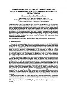
Fig. 4. The transform directions are chosen within each spatial segment of the size 16 × 16 so that the energy in the high-pass subbands is minimized allowing for the best matching with locally dominant directions in image. The set of chosen directions form the directional map. (a) The original image Lena. (b) The corresponding directional map. (c) The original image Baboon. (d) The corresponding directional map. indexed by n as d∗n = arg min d∈D

X

(d)

|Wn,i |2 ,

(2)

i (d)

where the wavelet coefficients Wn,i are produced by applying directionlets to the nth segment along the pair d of directions. The directional map determined by the set {d∗n } minimizes the energy in the high-pass subbands and provides the best matching between transform and locally dominant directions across segments. For the reason of simplicity of implementation, the pair of the horizontal and vertical directions is assigned by default to smooth segments with no apparent dominant direction (i.e. with low variation of the energy in the high-pass subbands for d ∈ D). Two examples of directional map are shown in Fig. 4 for the images Lena and Baboon. The concept of directional map is used in our interpolation algorithm to improve the extraction of edge information and the estimation of the HR wavelet subbands, as presented next. 3.2. Interpolation algorithm We propose a novel interpolation algorithm that uses the same concept as the previous method in [7] (revisited also in Section 2.1) with several modifications caused by implementation of directionlets instead of the 3-band 2-D WT. Similarly, the goal is, first, to estimate the corresponding wavelet subbands at HR and, then, to apply the inverse transform to obtain a reconstructed HR image. The estimation of the wavelet subbands also consists of the two phases: (a) initial estimate and (b) iterative POCS. In the initial estimate, the low-pass subband is bicubic-interpolated from the LR image, whereas the high-pass subbands are generated from the extracted SVP information. However, as opposed to the 3-band 2-D

(3)

By contrast to Chang et al., the SVP parameters, that is, the scaling constant Km and local Lipschitz regularity factor αm , are estimated in all the three high-pass subbands by linear regression using (3), instead of (1). The initially estimated HR subbands are iteratively refined in the second phase by projection onto three convex sets. The sets are defined by similar properties as in the original algorithm, with a modification for the first set that the subbands must belong to the corresponding subspace of directionlets, instead of the 3-band WT. Notice that the two SVP parameters that correspond to the same location estimated in different high-pass subbands are not independent, since they are produced by the same SVP. The relation among these values can be used to further improve the estimation of the HR high-pass subbands. However, we do not address this issue here and leave it for future work. The estimated HR subbands are transformed back to the original domain using inverse directionlets and the computed directional map. Notice also that the same transform is used in both the computation of directional map (as explained in Section 3.1) and the initial estimate of the high-pass subbands and, thus, this transform can be applied only once. This fact is exploited to reduce the overall computational complexity of the algorithm. 4. EXPERIMENTAL RESULTS We compare the performance of our method to the performance of both the traditional bicubic interpolation and the previous locally adaptive wavelet-based method from [7] applied to two test images, Lena and Baboon. To obtain peak signal-to-noise-ratio (PSNR), we first low-pass filter and subsample the original images and, then, we apply the interpolation algorithms to reconstruct the images at HR and to compare them to the original versions. Since the original source code for the method in [7] is not available, we have rewritten it and have obtained PSNRs that are not exactly equal to the results shown in the original paper, but approximately close. The LR 256 × 256 image Lena shown in Fig. 5(a) is interpolated to the size 512 × 512 pixels using the bicubic interpolation, wavelet-based and the method based on directionlets and the reconstructed images are shown in Fig. 5(b-d). The obtained numeric results are 30.62dB, 34.68dB and 35.43dB, respectively. Similarly, the numeric results for the image Baboon are 22.78dB, 23.61dB and 24.11dB for the three methods, as shown in Fig. 6. Notice that our interpolation algorithm significantly outperforms the other ones for both test images. Moreover, the visual quality of the interpolated images is evidently better because of sharper edges and texture. To emphasize this gain, the interpolated versions of the nose and mouth

of the baboon are zoomed in for all the three methods and shown in Fig. 1. 5. CONCLUSIONS

(a)

(b) PSNR=30.62dB

We have proposed a novel image interpolation algorithm obtained by implementation of directionlets in the previously proposed locally adaptive wavelet-based method. The algorithm adapts the transform directions to dominant directions across the image domain and successfully captures oriented features. Moreover, it extracts the information about these features (location, amplitude and degree of regularity) from the low-resolution image and uses these parameters to generate a high-resolution version with preserved sharpness. Our method outperforms the previous methods in terms of both numeric and visual quality of reconstructed images. The performance of the method can be even further improved by exploiting the relation of the extracted parameters across the wavelet subbands, which is left for future work. 6. REFERENCES

(c) PSNR=34.68dB

(d) PSNR=35.43dB

Fig. 5. The image Lena is interpolated from the size 256 × 256 to the size 512 × 512 pixels using the three methods: bicubic interpolation, wavelet-based and interpolation based on directionlets. (a) The LR image. (b) Bicubic interpolation (PSNR=30.62dB). (c) Locally adaptive wavelet-based interpolation [7] (PSNR=34.68dB). (d) Interpolation based on directionlets (PSNR=35.43dB).

[1] P. Th´evenaz, T. Blu, and M. Unser, “Interpolation revisited,” IEEE Trans. Med. Imag., vol. 19, pp. 739–758, July 2000. [2] K. Kinebuchi, D. D. Muresan, and T. W. Parks, “Image interpolation using wavelet-based hidden Markov trees,” Proc. ICASSP-2001, vol. 3, pp. 7–11, May 2001. [3] A. Temizel, “Image resolution enhancement using wavelet domain hidden Markov tree and coefficient sign estimation,” Proc. ICIP-2007, vol. 5, pp. 381–384, Sept. 2007. [4] M. Li and T. Nguyen, “Markov random field model-based edge-directed image interpolation,” Proc. ICIP-2007, vol. 2, pp. 93–96, Sept. 2007. [5] J. Allebach and P. Wong, “Edge-directed interpolation,” Proc. ICIP-1996, vol. 3, pp. 707–710, Sept. 1996. [6] X. Li and M. T. Orchard, “New edge-directed interpolation,” IEEE Trans. Image Processing, vol. 10, pp. 1521–1527, Oct. 2001. [7] S. Grace Chang, Z. Cvetkovi´c, and M. Vetterli, “Locally adaptive wavelet-based image interpolation,” IEEE Trans. Image Processing, vol. 15, pp. 1471–1485, June 2006.

(a)

(b) PSNR=22.78dB

[8] S. Mallat and S. Zhong, “Characterization of signals from multiscale edges,” IEEE Trans. Pattern Anal. Machine Intell., vol. 14, pp. 2207–2232, July 1992. [9] S. Mallat, A Wavelet Tour of Signal Processing, Academic Press, San Diego, CA, 1997. [10] V. Velisavljevi´c, B. Beferull-Lozano, and M. Vetterli, “Spacefrequency quantization for image compression with directionlets,” IEEE Trans. Image Processing, vol. 16, pp. 1761–1773, July 2007.

(c) PSNR=23.61dB

(d) PSNR=24.11dB

Fig. 6. The image Baboon is interpolated using the same three methods. (a) The LR image. (b) Bicubic interpolation (PSNR=22.78dB). (c) Locally adaptive wavelet-based interpolation [7] (PSNR=23.61dB). (d) Interpolation based on directionlets (PSNR=24.11dB).

[11] V. Velisavljevi´c, B. Beferull-Lozano, and M. Vetterli, “Spacefrequency quantization using directionlets,” Proc. ICIP-2007, vol. 3, pp. 161–164, Sept. 2007. [12] M. Antonini, M. Barlaud, P. Mathieu, and I. Daubechies, “Image coding using wavelet transform,” IEEE Trans. Image Processing, vol. 1, pp. 205–220, Apr. 1992.