Resampling Method For Unsupervised Estimation Of Cluster Validity

arXiv:physics/0005046v1 [physics.comp-ph] 18 May 2000

Resampling Method For Unsupervised Estimation Of Cluster Validity Erel Levine and Eytan Domany Department of Physics of Complex Systems, The Weizmann Institute of Science, Rehovot 76100, Israel February 2, 2008 Abstract We introduce a method for validation of results obtained by clustering analysis of data. The method is based on resampling the available data. A figure of merit that measures the stability of clustering solutions against resampling is introduced. Clusters which are stable against resampling give rise to local maxima of this figure of merit. This is presented first for a one-dimensional data set, for which an analytic approximation for the figure of merit is derived and compared with numerical measurements. Next, the applicability of the method is demonstrated for higher dimensional data, including gene microarray expression data.

1

Introduction

Cluster analysis is an important tool to investigate and interpret data. Clustering techniques are the main tool used for exploratory data analysis, namely when one is dealing with data about whose internal structure little or no prior information is available. Cluster algorithms are expected to produce partitions that reflect the internal structure of the data and identify “natural” classes and hierarchies present in it. Throughout the years a wide variety of clustering algorithms have been proposed. Some algorithms have their origins in graph theory, whereas others are based on statistical pattern recognition, selforganization methods and more. More recently, several algorithms, which are rooted in statistical mechanics, have been introduced. Comparing the relative merits of various methods is made difficult by the fact that when applied to the same data set, different clustering algorithms often lead to markedly different results. In some cases such differences are expected, since different algorithms make different (explicit or implicit) assumptions about the structure of the data. If the particular set that is being studied consists, for example, of several clouds of data point, with each cloud spherically distributed about its center, methods that assume such structure (e.g. k-means), will work well. On the other hand, if the data consist of a single non-spherical cluster, the same algorithms will fare miserably, breaking it up into a hierarchy of partitions. Since for the cases of interest one does not know which assumptions are satisfied by the data, a researcher may run into severe difficulties in interpretation of his results; by preferring one algorithm’s clusters over those of another, he may re-introduce his biases about the underlying structure - precisely those biases, which one hoped to eliminate by employing clustering techniques. In addition, the differences in the sensitivity of different algorithms to noise, which inherently exists in the data, also yield a major contribution to the difference between their results. The ambiguity is made even more severe by the fact that even when one sticks exclusively to one’s favorite algorithm, the results may depend strongly on the values assigned to various parameters of the particular algorithm. For example, if there is a parameter which controls the resolution at which the data are viewed, the algorithm produces a hierarchy of clusters (a dendrogram) as a function of this parameter. One then has to decide which level of the dendrogram reflects best the “natural” classes present in the data? Needless to say, one wishes to answer these questions in an unsupervised manner, i.e. making use of nothing more than the available data itself. Various methods and indicators, that come under the name “cluster validation”, attempt to evaluate the results of cluster analysis in this manner (Jain and Dubes, 1988). Numerous studies suggest direct and indirect indices for evaluation of hard clustering (Jain and Dubes, 1988; Bock, 1985), probabilistic clustering (Duda and Hart, 1973), and fuzzy clustering (Windham, 1982; Pal and Bezdek, 1995) results. Hard clustering indices are often based on some geometrical motivation to estimate how compact and well separated the clusters are (e.g. Dunn’s index 1

0.8

0.8

(a)

0.6

0.6

0.4

0.4

0.2

0.2

0

0

−0.2

−0.2

−0.4

−0.4

−0.6

−0.6

−0.8

−0.8 −0.5

0

0.5

(b)

−0.5

0

0.5

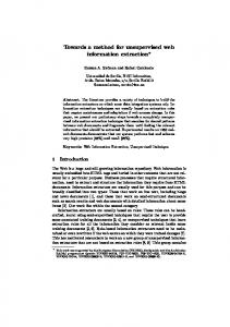
Figure 1: Two samples, drawn from an 8-shaped uniform distribution. Sample (a) is somewhat nontypical. (Dunn, 1974) and its generalizations (Bezdek and Pal, 1995)); others are statistically motivated (e.g. comparing the within cluster scattering with the between-cluster separation (Davies and Bouldin, 1979)). Probabilistic and fuzzy indices are not considered here. Indices proposed for these methods are based on likelihood-ratio tests (Duda and Hart, 1973), information-based criteria (Cutler and Windham, 1994) and more. Another approach to cluster validity includes some variant of cross-validation (Fukunaga, 1990). Such methods were introduced both in the context of hard clustering (Jain and Moreau, 1986) and fuzzy clustering (Smyth, 1996). The approach presented here falls into this category. In this paper we present a method to help select which clustering result is more reliable. The method can be used to compare different algorithms, but it is most suitable to identify, within the same algorithm, those partitions that can be attributed to the presence of noise. In these cases a slight modification of the noise may alter the cluster structure significantly. Our method controls and alters the noise by means of resampling the original dataset. In order to illustrate the problem we wish to address and its proposed solution, consider the following example. Say a scientist is investigating mice, and comes to suspect that there are several types of them. She therefore measures two features of the mice (such as weight and shade), looks for clusters in this two-dimensional data set, and indeed finds two clusters. She can therefore conclude that there are two types of mice in her lab. Or can she? Imagine that the data collected by the scientist can be represented by the points on figure 1 (a). This data set was in fact taken from a shaped uniform distribution (with a relatively narrow “neck” at the middle). Hence no partition really exists in the underlying structure of the data and, unless one makes explicit assumptions about the shape of the data clouds, one should identify a single cluster. The particular cluster algorithm used breaks, however, the data into two clusters along the horizontal gap seen in figure 1 (a). This gap happens to be the result of fluctuations in the data, or noise in the sampling (or measurement) process. More typical data sets, such as that of figure 1 (b), do not have such gaps and are not broken into two clusters by the algorithm. If more than a single sample had been available, it would have been safe to assume that this particular gap would not have had appeared in most samples. The partition into two clusters would, in that case, be easily identified as unreliable. In most cases, however, only a single sample is available, and resampling techniques are needed in order to generate several ones. In this paper we propose a cluster validation method which is based on resampling (Good, 1999; Efron and Tibshirani, 1993): subsets of the data under investigation are constructed randomly, and the cluster algorithm is applied to each subset. The resampling scheme is introduced in Sec. 2, and a figure of merit is proposed to identify the stable clustering solutions, which are less likely to be the results of noise or fluctuations. The proposed procedure is tested in Sec. 3 on a one-dimensional data set, for which an analytical expression for the figure of merit is derived and compared with the corresponding numerical results. In Sec. 4 we demonstrate the applicability of our method to two artificial data sets (in d = 2 dimensions) and to real (very high dimensional) DNA microarray data.

2

2

The Resampling Scheme

Let us denote the number of data points in the set to be studied by N . Typically, application of any cluster algorithm necessitates choosing specific values for some parameters. The results yielded by the clustering algorithm may depend strongly on this choice. For example, some algorithms (e.g. the c-shell fuzzy-clustering (Bezdek, 1981) and the iso-data algorithm (Cover and Thomas, 1991)) take the expected number of clusters as part of their input. Other algorithms (e.g. Valley-Seeking (Fukunaga, 1990)) have the number of neighbors of each point as an external parameter. In particular, many algorithms have a parameter that controls the resolution at which clusters are identified. In agglomerative clustering methods, for example, this parameter defines the level of the resulting dendrogram at which the clustering solution is identified (Jain and Dubes, 1988). For the K-nearest-neighbor algorithm (Fukunaga, 1990) a change in the number of neighbors of each point, K, controls the resolution. For Deterministic Annealing and the Superparamagnetic Clustering (SPC) algorithm this role is played by the temperature T. As this control parameter is varied, the data-points get assigned to different clusters, giving rise to a hierarchy. At the lowest resolution all N points belong to one cluster, whereas at the other extreme one has N clusters, of a single point in each. As the resolution parameter varies, clusters of data points break into sub-clusters which break further at a higher level. Sometimes the aim is to generate precisely such a dendrogram. In other cases one would like to produce a single partitioning of the data, which captures a particular important aspect. In such a case we wish to identify that value of the resolution control parameter, at which the most reliable, natural clusters appear. In these situations the resolution parameter plays the role of one (probably the most important) member of the family of parameters of the algorithm that needs to be fixed. Let us denote the full set of parameters of our algorithm by V . Any particular clustering solution can be presented in the form of an N × N cluster connectivity matrix Tij , defined by  1 points i and j belong to the same cluster Tij = (1) 0 otherwise In order to validate this solution, we construct an ensemble of m such matrices, and make comparisons among them. This ensemble is created by constructing m resamples of the original data set. A resample is obtained by selecting at random a subset of size f N of the data points. We call 0 ≤ f ≤ 1 the dilution factor. We apply to every one of these subsets the same clustering procedure, that was used on the full dataset, using the same set of parameters V . This way we obtain for each resample µ, µ = 1, ...m, its own clustering results, summarized by the f N × f N matrix T (µ) . We define a figure of merit M(V ) for the clustering procedure (and for the choice of parameters) that we used. The figure of merit is based on comparing the connectivity matrices of the resamples, T (µ) (µ = 1 . . . m), with the original matrix T : M(V ) =≪ δTij ,T (µ) ≫m ,

(2)

ij

The averaging implied by the notation ≪ · ≫m is twofold. First, for each resample µ we average over all those pairs of points ij which were neighbors1 in the original sample, and have both survived the resampling. Second, this average value is averaged over all the m different resamples. Clearly, 0 ≤ M ≤ 1, with M = 1 for perfect score. The figure of merit M measures the extent to which the clustering assignments obtained from the resamples agrees with that of the full sample. An important assumption we have made implicitly in this procedure is that the algorithm‘s parameters are “intensive”, i.e. their effect on the quality of the result is independent of the size of the data set. We can generalize our procedure in several ways to cases when this assumption does not hold2 (Levine, 2000). After calculating M(V ), we have to decide whether we accept the clustering result, obtained using a particular value of the clustering parameters, or not. For very low and very high values of M the decision may be easy, but for mid-range values we may need some additional information to guide our decision. In such a case, the best way to proceed is to change the values of the clustering parameters, and go through the whole process once again. Having done so for some set parameter choices V , we study the way M(V ) varies as a function of V . Optimal sets of parameters V ∗ are identified by locating the maxima of this function. It should be noted, 1 For

various definition of neighbors see (Fukunaga, 1990) For example, we can define our figure of merit on the basis of pairwise comparisons of our resamples, and find an optimal set of parameters V1∗ in the way explained below. Next, we look for parameters V2∗ for which clustering of the full sample yields closest results to those obtained for the resamples (clustered at V1∗ ). 2

3

however, that some of these maxima are trivial and should not be used. Examples that demonstrate this point are presented in the next section. Our procedure can be summarized in the following algorithmic form: Step 0. Choose values for the parameters V of the clustering algorithm. Step 1. Perform clustering analysis of the full data set. Step 2. Construct m sub sets of the data set, by randomly selecting f N of the N original data-points. Step 3. Perform clustering analysis for each sub set. Step 4. Based on the clustering results obtained in Steps 1 and 3 calculate M(V ), as defined in eq. (2). Step 5. Vary the parameters V and identify stable clusters as those for which a local maximum of M is observed.

3

Analysis of a One Dimensional Model

To demonstrate the procedure outlined above we consider a clustering problem, which is simple enough to allow an approximate analytical calculation of the figure of merit M and its dependence on a parameter that controls the resolution. Consider a one dimensional data set which consists of points xi , i − 1, ..., N , selected from two identical but displaced uniform distributions, such as the one shown in Fig. 3. The distributions are characterized by the mean distance between neighboring points, d = 1/λ, and the distance or gap between the two distributions, ∆. Distances between neighboring points within a cluster are distributed according to the Poisson distribution, P (s) = λe−λs ds.

(3)

The results of a clustering algorithm that reflects the underlying distribution from which the data were selected should identify two clusters in this data set. Consider a simple nearest-neighbor clustering algorithm, which assigns two neighboring points to the same cluster if and only if the distance between the two is smaller than a threshold a. Clearly, α = λa is the dimensionless parameter of the algorithm that controls the resolution of the clustering. For very small α > 1, all pairs of neighbors are assigned to the same cluster, and hence all points reside in one cluster. Starting from α >> 1 and reducing it gradually, one generates a dendrogram. At an intermediate value of α we may get any number of clusters between one and N . Hence, if we picked some particular value of α at which we obtained some clusters, we must face the dilemma of deciding whether these clusters are “natural”, or are the result of the fluctuations (i.e. noise) present in the data. In other words, we would like to validate the clustering solution obtained for the full data set for a given value of α. We do this using the resampling scheme described above. A resample is generated by independently deciding for each data point whether it is kept in the resample (with probability f ), or is discarded (with probability 1 − f ). This procedure is repeated m times, yielding m resamples. All length scales of the original problem get rescaled by the resampling procedure by a factor of 1/f ; the mean distance between neighboring points in the resampled set is d′ = 1/λf , and the distance between the two uniform distributions is ∆′ = ∆/f . Clustering is therefore performed with a rescaled threshold a′ = a/f on any resample; the resolution parameter keeps its original value, α′ = a′ /d′ = α. We first wish to get an approximate analytical expression for the figure of merit M(α) described above. To do this we consider the gaps between data points, rather then the points themselves. Let us denote by b the distance between the data point i (of the original sample) and its nearest left neighbor: b = xi − xi−1 , with the two points on the same side of the gap ∆. We first assume that this edge is not broken by the clustering algorithm, b < a. Given a resample that includes point i, we define b′ in the same fashion. The new, resampled left neighbor of i resides in the same cluster as i if b′ < a′ ; the probability that this happens is given by (Levine, 2000) ∞ X f 2 (1 − f )m−1 γ(m, α/f − β). P1 (β) = (m − 1)! m=1

4

(4)

where the dimensionless variable β = λb was introduced. Here γ(n, z) is Euler’s incomplete Gamma function, Z z γ(n, z) = e−t tn−1 dt, (5) 0

except that in our convention, we take γ(n, z < 0) = γ(n, 0). Similarly, if points i and i − 1 were not assigned to the same cluster in the original sample, then the probability that the same would happen in a resample is(Levine, 2000) ∞ X f 2 (1 − f )m−1 Γ(m, α/f − β), P2 (β) = (m − 1)! m=1

where Γ(n, z) is the other incomplete Gamma function, Z ∞ Γ(n, z) = e−t tn−1 dt,

(6)

(7)

z

and we take Γ(n, z < 0) = Γ(n, 0) = (n − 1)!, so Bm = 1 for α ≤ f β. We now calculate the index M in an approximate manner, by averaging P1 and P2 over all edges. This calculation matches the definition (2) of M in spirit. For pairs residing within a true cluster, the averaging is done by integrating over all possible values of b; Z α Z ∞ −β A(α) = e P1 (β) dβ + e−β P2 (β) dβ . (8) 0

α

For pairs which lie of different sides of the gap, we should only compare a with the size of the gap ∆ :  P1(δ) α ≥ δ , (9) Bδ (α) = P2(δ) α < δ where the dimensionless variable δ = λ∆ was introduced. Clearly, in the one-dimensional example there are much fewer edges of the second kind than of the first. This, however, is not the case for data in higher dimensions, so we give equal weights to the two terms A and B 3 1 [A(α) + Bδ (α)] . (10) 2 We now plot M as a function of the resolution parameter α for both f = 1/2 and f = 2/3 (figure 2(a)), assuming the inter-cluster distance δ = 5. A clear peak can be observed in both curves at α ≃ 2.5 and α ≃ 3.3, respectively. Similarly, for δ = 10 clear peaks are identified at α ≃ 5 and α ≃ 7 (figure 2(b)). As we will see, these peaks correspond to the most stable clustering solution, which indeed recovers the original clusters. The trivial solutions, of a single cluster (of all data points) and the opposite limit of N single-point clusters, are also stable, and appear as the maxima of M(α) at α > 1, respectively. In order to test how good is our analytic approximate evaluation of M, we clustered a one-dimensional data set of figure 3(a), and calculated the index M as defined in eq. (2). The data set consists of N = 200 data points sampled from two uniform distribution of mean nearest neighbor distance 1/λ = 1 and shifted by ∆ = 10. The dendrogram obtained by varying α is shown in Fig. 3(c). It clearly exhibits two stable clusters; stability is indicated by the wide range of values of α over which the two clusters “survive”. Next, we generated 100 resamples of size 130 (i.e. f ≈ 2/3), and applied the geometrical clustering procedure described above to each resample. By averaging over the different resamples the figure of merit M was calculated for different values of the dimensionless resolution parameter α, as shown in figure 3(b). The peak between α ≈ 4 and α ≈ 7, corresponding to the most stable, “correct” clustering solution, is clearly identified. The agreement between our approximate analytical curve of figure 2(b) for M (α) and the numerically obtained exact curve of figure 3(b) is excellent and most gratifying. M(α) =

3 The ratio between the two terms is of the order (d − 1)/d, where d is the dimensionality of the problem. For high dimensional problems, this ratio is close to 1.

5

0.9

0.9

0.8

0.8

M

1

M

1

0.7

0.7

0.6

0.6

(a) 0.5 0

(b)

f=1/2 f=2/3 2

4

6

α

f=1/2 f=2/3

0.5

8

10

0

5

α

10

15

Figure 2: Mean behavior of M as a function of the geometric threshold, according to equation (10), for two clusters. The function is evaluated for the inter-cluster distances (a) ∆ = 5λ and (b) ∆ = 10λ, with dilution parameters f = 1/2 and f = 2/3.

12 1

10 0.9

8

M

0.8

6

0.7

4 0.6

2 0.5

0

0

0

0.5

1

1.5

2

2

4

6

α

2.5

(a)

8

10

12

(b)

1

2

3

4

α

5

6

7

8

9 20

40

60

80

100

120

140

160

180

200

Data Points (c)

Figure 3: Resampling results for a one-dimensional data set. 200 points were chosen uniformly from two clusters, separated by ∆λ = 10. Histogram of the data is given in (a). We performed 100 resamples of 130 points, (i.e. f ≈ 2/3) to calculate M. In (b) we plot M as a function of the resolution parameter α. The peak between α ≈ 4 and α ≈ 7 corresponds to the correct two cluster solution, as can be seen from the dendrogram shown in (c).

6

4

3

2

1

0

−1

−2

−3

−4 −5

−4

−3

−2

−1

0

1

2

3

4

5

Figure 4: The three-ring problem. 1400 points are sampled from a three a three-component distribution described in the text. 900

Outer ring

800

700

Cluster size

600

500

Middle ring

400

300

Inner ring

200

100

0

0

0.02

0.04

0.06

0.08

0.1

0.12

0.14

0.16

0.18

Temperature

Figure 5: Clustering solution of the three ring problem as a function of resolution parameter (the temperature).

4 4.1

Applications Two Dimensional Toy Data

The analysis of the previous section predicts a typical behavior of M as a function of the parameters that control resolution; in particular, it suggests that one can identify a stable, “natural” partition as the one obtained at a local maximum of the function M. This prediction was based on an approximate analytical treatment and backed up by numerical simulations of one-dimensional data. Here we demonstrate that this behavior is also observed for a toy problem which consists of the two-dimensional data set shown in figure 4. The angular coordinates of the data points are selected from a uniform distribution, θ ∼ U[0, 2π]. The radial coordinates are normal distributed, r ∼ N[R, σ] around three different radii R. The outer “ring” (R = 4.0, σ = 0.2) consists of 800 points, and the inner “rings” (R = 2.0, 1.0, σ = 0.1) consists of 400 and 200 points, respectively. The algorithm we choose to work with is the super-paramagnetic clustering (SPC) algorithm, recently introduced by Blatt et al. (Blatt et al., 1996; Domany, 1999). This algorithm provides a hierarchical clustering solution. A single parameter T , called “temperature”, controls the resolution : higher temperatures corresponds to higher resolutions. Variation of T generates a dendrogram. The outcome of the algorithm depends also on an additional parameter K, described below in subsection 4.3.1. The data of Fig. 4 were clustered with K = 20. The results of the clustering procedure are presented in Figure 5. A stable phase, in which the three rings are clearly identified appears at the temperature range 0.3 ≤ T ≤ 0.8. In order to identify the value of T that yields the “correct” solution, we generated and clustered 20 different resamples from this toy data set, with a dilution factor of f = 2/3. The resolution parameter (temperature) of each resample was rescaled so that the transition temperature at which the single large cluster breaks up agrees with the temperature of the same transition in the original sample. The function M(T ), plotted in figure 6, exhibits precisely the expected behavior, with two trivial maxima and an additional one at T = 0.05. This value indeed corresponds to the “correct” solution, of three clusters.

7

1.05

1

0.95

M

0.9

0.85

0.8

0.75

0.7

0.65

0

0.02

0.04

0.06

0.08

0.1

0.12

0.14

0.16

0.18

0.2

Temperature

Figure 6: M as a function of the temperature for the three-ring problem. 1.05

1.05

1

1

0.95 0.95 0.9 0.9

M

M

0.85 0.8

0.85

0.75 0.8 0.7 0.75

0.65 0.6 0

0.02

0.04

0.06

0.08

0.1

0.12

0.14

0.7 0

0.16

Temperature

50

100

150

200

Number of cluster merges

Figure 7: M as a function of the resolution parameter for the single-cluster problem. Clustering is performed using the SPC algorithm (left) and the Average-Linkage algorithm (right).

4.2

A Single Cluster – Dealing With Cluster Tendency

A frequent problem of clustering methods is the so called ’cluster tendency’; that is, the tendency of the algorithm to partition any data, even when no natural clusters exist. In particular, agglomerative algorithms, which provide a hierarchy of clusters, always generate some hierarchy as a control parameter is varied. We expect this hierarchy to be very sensitive to noise, and thus unstable against resampling. We tested this assumption for the data set of figure 1(a). The test was performed using two clustering methods: the SPC algorithm mentioned above, and the Average-Linkage clustering algorithm. The latter is an agglomerative hierarchical method. It starts with N distinct clusters, one for each point, and forms the hierarchy by successively merging the closest pair of clusters, and redefining the distance between all other clusters and the new one. This step is repeated N − 1 times, until only a single element remains. The output of this hierarchical method is a dendrogram. For more details see (Jain and Dubes, 1988). We performed our resampling scheme with m = 20 resamples and dilution factor of f = 2/3, for different levels of resolution. The results are shown in figure 7. The only stable solutions identified by both algorithms are the trivial ones, of either a single cluster or N clusters. In this case, obviously, the single cluster solution is also the natural one.

4.3

Clustering DNA Microarray Data

We turn now to apply our procedure to real-life data. We present here validation of cluster analysis performed for DNA Microarray Data. Gene-array technology provides a broad picture of the state of a cell by monitoring the expression levels of thousands of genes simultaneously. In a typical experiment simultaneous expression levels of thousands of genes are viewed over a few tens of cell cultures at different conditions. For details see (Chee et al., 1996; Brown and Botstein, 1999). The experiment whose analysis is presented here is on colon cancer tissues(Alon et al., 1999). Expression levels of ng = 2000 genes were measured for nt = 62 different tissues, out of which 40 were tumor tissues and 22 were normal ones. Clustering analysis of such data has two aims: (a) Searching for groups of tissues with similar gene expression profiles. Such groups may correspond to normal vs tumor tissues. For this analysis the nt tissues are considered as the data points, embedded in an ng dimensional space. 8

1

0.95

0.9

0.85

M

0.8

0.75

0.7

0.65

0.6

0.55

0.5

0

5

10

15 K

20

25

30

Figure 8: Figure of merit M as a function of K for the colon tissue data. (b) Searching for groups of genes with correlated behavior. For this analysis we view the genes as the data points, embedded in an nt dimensional space and we hope to find groups of genes that are part of the same biological mechanism. Following Alon et al. , we normalize each data point (in both cases) such that the standard deviation of its components is one and its mean vanishes. This way the Euclidean distance between two data points is trivially related to the Pearson correlation between the two. 4.3.1

Clustering tissues

The main purpose of this analysis is to check whether one can distinguish between tumor and normal tissues on the basis of gene expression data. Since we know in what aspect of the data’s structure we are interested, in this problem the working resolution is determined as the value at which the data first breaks into two (or more) large clusters (containing, say, more than ten tissues). There may be, however, other parameters for the clustering algorithm, which should be determined. For example, the SPC algorithm has a single parameter K, which determines how many data points are considered as neighbors of a given point. The algorithm places edges or arcs that connect pairs of neighbors i, j, and assigns a weight Jij to each edge, whose value decreases with the distance |~xi − ~xj | between the neighboring data-points. Hence the outcome of the clustering process may depend on K, the number of neighbors connected to each data point by an edge. We would like to use our resampling method to determine the optimal value for this parameter. We clustered the tissues, using SPC, for several values of K. For each case we identified the temperature at which the first split to large clusters occurred. For each case we performed the same resampling scheme, with m = 20 resamples of size 23 nt , and calculated the figure of merit M(K). The results obtained for several values of K are plotted in figure 8. Very low and very high values of K give similarly stable solutions. In the low-K case each point is practically isolated, and the data breaks immediately into microscopic clusters. The high-K case is just the opposite – each points is considered “close” to very many other points, and no macroscopic partition can be obtained. At K = 8 we observe, however, another peak in M. At this K the clustering algorithm yields indeed two large clusters, which correspond to the two “correct” clusters of normal and tumor tissues, as shown on Fig. 9. Such solutions appear also for some higher values of K, but in these cases the clusters are not stable against resampling. 4.3.2

Clustering genes

Cluster analysis of the genes is performed in order to identify groups of genes which act cooperatively. Having identified a cluster of genes, one may look for a biological mechanism that makes their expression correlated. Trying to answer this question, one may, for example, identify common promoters of these genes (Getz et al., 2000b). One may also use one or more clusters of genes to reclassify the tissues (Getz et al., 2000a), looking for clinical manifestations associated with the expression levels of the selected groups of genes. Therefore in this case it is important to assess the reliability of each particular gene cluster separately.

9

Figure 9: Clustering of the tissues, using K=8. Leaves of the tree are colored according to the known classification to normal (dark) and tumor (light). The two large clusters marked by arrows recover the tumor/normal classification. The SPC clustering algorithm was used to cluster the genes. A resulting dendrogram is presented in Fig. 10, in which each box represents a cluster of genes. Our resampling scheme has been applied to this data, using m = 25 resamples of size 1200 ( f = 0.6). This time, however, we calculated M(C), for each cluster C of the full original sample, separately. That is, we calculated M only for the points of a single cluster C, at the temperature at which it was identified, and then moved on to the next cluster. We therefore get a stability measure for each cluster. Next, we focus our attention on clusters of the highest scores. First, we considered the top 20 clusters. If one of these clusters is a descendent of another one from the list of 20, we discard it. After this pruning we were left with 6 clusters, which are circled and numbered in figure 10 (the numbers are not related to the stability score). We are now ready to interpret these stable clusters. The first three consist of known families of genes. #1 is a cluster Ribosomal proteins. The genes of cluster #2 are all Cytochrome C genes, which are involved in energy transfer. Most of the genes of cluster #3 belong to the HLA-2 family, which are histocompatability antigens. Cluster #4 contains a variety of genes, some of which are related to metabolism. When trying to cluster the tissues based on these genes alone, we find a stable partition to two clusters, which is not consistent with the tumor/normal labeling. At this point, we are still unable to explain this partition. Clusters #5 and #6 also contain genes of various types. The genes of these clusters have most typical behavior: all the genes of cluster #5 are highly expressed in the normal tissues but not in the tumor ones; And all genes of cluster #6 are the other way around. To summarize, clustering stability score based on resampling enabled us to zero in on clusters with typical behavior, which may have biological meaning. Using resampling enabled us to select clusters without making any new assumption, which is a major advantage in exploratory research. The downside of this method, however, is it’s computational burden. In this experiment we had to perform clustering analysis 20 times for a rather large data set. This would be the typical case for DNA microarray data.

5

Discussion

This work proposes a method to validate clustering analysis results, based on resampling. It is assumed that a cluster which is robust to resampling is less likely to be the result of a sample artifact or fluctuations. The strength of this method is that it requires no additional assumptions. Specifically, no assumption is made either about the structure of the data, the expected clusters, or the noise in the data. No information, except the available data itself, is used. We introduced a figure of merit, M, which reflects the stability of the cluster partition against resampling. The typical behavior of this figure of merit as a function of the resolution parameter allows clear identification of natural resolution scales in the problem. The question of natural resolution levels is inherent to the clustering problem, and thus emerges in any clustering scheme. The resampling method introduced here is general, and applicable to any kind of data set, and to any clustering algorithm.

10

90

80

70

1

4

60

5

6 2

50

40

30

20

200

400

600

800

1000

1200

1400

1600

1800

2000

Figure 10: Dendrogram of genes. Clusters of size 7 or larger are shown as boxes. Selected clusters are circled and numbered, as explained in the text.

11

For a simple one-dimensional model we derived an analytical expression for our figure of merit and its behavior as a function of the resolution parameter. Local maxima were identified for values of the parameter corresponding to stable clustering solutions. Such solutions can either be trivial (at very low and very high resolution); or non-trivial, revealing genuine internal structure of the data. Resampling is a viable method provided the original data set is large enough, so that a typical resample still reflects the same underlying structure. If this is the case, our experience shows that a dilution factor of f ≃ 2/3 works well for both small and large data sets.

Acknowledgments This research was partially supported by the Germany - Israel Science Foundation (GIF). We thank Ido Kanter and Gad Getz for discussions.

References Alon, U. et al. (1999). Broad patterns of gene expression revealed by clustering analysis of tumor and normal colon tissues probed by oligonucleotide arrays. Proc. Natl Acad. Sci. USA, 96:6745–6750. Bezdek, J. (1981). Pattern Recognition with Fuzzy Objective Function Algorithms. Plenum Press, New York. Bezdek, J. and Pal, N. (1995). Cluster validation with generalized dunn’s indeices. Proc. 1995 2nd NZ int’l., pages 190–193. Blatt, M., Wiseman, S., and Domany, E. (1996). Super–paramagnetic clustering of data. Physical Review Letters, 76:3251–3255. Bock, H. (1985). On significance tests in cluster analysis. J. Classification, 2:77–108. Brown, P. and Botstein, D. (1999). Exploring the new world of the genome with dna microarrays. Nature Genetics, 21:33 – 37. Chee, M. et al. (1996). Accessing genetic information with high-density dna arrays. Science, 274:610–614. Cover, T. and Thomas, J. (1991). Elements of Information Theory. Wiley–Interscience, New York. Cutler, A. and Windham, M. (1994). Information-based validity functionals for mixture analysis. Proc. 1st US/Japan conf. on frontiers in statistical modeling, pages 149–170. Davies, D. and Bouldin, D. (1979). A cluster separation measure. IEEE trans. PAMI, pages 224–227. Domany, E. (1999). Super-paramagnetic clustering of data – the definitive solution of an ill-posed problem. Physica A, 263:158. Duda, R. and Hart, P. (1973). Pattern Classification and Scene Analysis. Wiley–Interscience, New York. Dunn, J. (1974). A fuzzy relative isodata process and its use in detecting compact well-separated clusters. J. Cybernetics, 3:32–57. Efron, B. and Tibshirani, R. (1993). An Introduction to the Bootstrap. Chapman & Hall. Fukunaga, K. (1990). Introduction to statistical Pattern Recognition. Academic Press, San Diego. Getz, G., Levine, E., and Domany, E. (2000a). Coupled two-way clustering of dna microarry data. physics/0004009. Getz, G., Levine, E., Domany, E., and Zhang, M. (2000b). Super-paramagnetic clustering of yeast gene expression profiles. physics/9911038. Good, P. (1999). Resampling methods. Springer-Verlag, New York. Jain, A. and Dubes, R. (1988). Algorithms for Clustering Data. Prentice–Hall, Englewood Cliffs. Jain, A. and Moreau, J. (1986). Bootstrap technique in cluster analysis. Pattern Recognition, 20:547–569. Levine, E. (2000). Unsupervised estimation of clsuter validity – Methods and Applications. M.Sc. Thesis, The Weizmann Inst. of Science. Pal, N. and Bezdek, J. (1995). On cluster validity for the fuzzy c-means model. IEEE trans. Fuzzy Systems, 3:370–376. Smyth, P. (1996). Clustering using monte carlo cross-validation. KDD-96 Proceedings, Second International Conference on Knowledge Discovery and Data Mining, pages 126–133. Windham, M. (1982). Cluster validity for the fuzzy c-means clustering algorithm. IEEE trans. PAMI, 4:357–363.

12