Hindawi Mathematical Problems in Engineering Volume 2018, Article ID 3757580, 11 pages https://doi.org/10.1155/2018/3757580
Research Article A Fuzzy Co-Clustering Algorithm via Modularity Maximization Yongli Liu
, Jingli Chen
, and Hao Chao
School of Computer Science and Technology, Henan Polytechnic University, Jiaozuo 454003, Henan, China Correspondence should be addressed to Yongli Liu;
[email protected] Received 3 September 2018; Accepted 21 October 2018; Published 29 October 2018 Academic Editor: Francesco Lolli Copyright © 2018 Yongli Liu et al. This is an open access article distributed under the Creative Commons Attribution License, which permits unrestricted use, distribution, and reproduction in any medium, provided the original work is properly cited. In this paper we propose a fuzzy co-clustering algorithm via modularity maximization, named MMFCC. In its objective function, we use the modularity measure as the criterion for co-clustering object-feature matrices. After converting into a constrained optimization problem, it is solved by an iterative alternative optimization procedure via modularity maximization. This algorithm offers some advantages such as directly producing a block diagonal matrix and interpretable description of resulting co-clusters, automatically determining the appropriate number of final co-clusters. The experimental studies on several benchmark datasets demonstrate that this algorithm can yield higher quality co-clusters than such competitors as some fuzzy co-clustering algorithms and crisp block-diagonal co-clustering algorithms, in terms of accuracy.
1. Introduction Co-clustering, also called biclustering or block-clustering, aiming to group a set of objects and a set of features simultaneously, has found an increasingly wide utilization in many fields. In the bioinformatics domain, co-clustering method has been used for simultaneously clustering genes and conditions [1]. Hussain and Ramazan [2] referred the theory of co-clustering text data and proposed a new algorithm based on weighted similarity, which generated two co-similarity matrices between genes and between conditions. In collaborative filtering, co-clustering technique is commonly used to simultaneously cluster users and items [3]. Honda et al. [4] utilized the sequential weighted coclustering approach to find user-item co-clusters and recommended the proper items to the users according to the membership of users and items. In text mining, coclustering algorithms are devoted to grouping documents and words simultaneously [5]. Tjhi and Chen [6] proposed a new fuzzy co-clustering algorithm for documents and words based on Ruspini’s condition. The proposal improved the drawback of some previous co-clustering algorithms about the constraint for word memberships, which caused the failure to obtain practical and valuable natural fuzzy word clusters.
Fuzzy co-clustering further extends co-clustering by adding fuzzy membership function. It therefore simultaneously keeps advantages of co-clustering and fuzzy clustering, including dimensionality reduction, interpretable clusters, and improvement in accuracy [7]. In a fuzzy co-clustering framework, the fuzzy relationship is presented by the captured degree to which objects belong to each other, as well as the features. Based on the fuzzy relationship, the objective function is designed, which will be minimized or maximized through multiple iterations until the convergence is realized. Oh et al. [8] proposed the famous fuzzy clustering algorithm for categorical multivariate data (FCCM), which maximizes the co-occurrence of categorical attributes and the individual patterns in clusters. Kummamuru et al. [9] modified the FCCM algorithm so that it can be used to cluster large text corpora. Hanmandlu et al. [10] presented a novel fuzzy coclustering algorithm for images color segmentation, named FCCI. The FCCI formulates an objective function which contains a multidimensional distance function as the dissimilarity measure and entropy as the regularization term. Forsati et al. [11] introduced a new fuzzy co-clustering approach based on genetic algorithm, computed the similarity between web pages and users, and proposed recommendations for hybrid recommender systems. These works show that fuzzy co-clustering can always achieve higher clustering accuracy,
2
Mathematical Problems in Engineering
because of its fuzzy mathematical method which determines the fuzzy relationship among samples. Although fuzzy co-clustering algorithms could be simultaneously carried out on both the object and feature dimensions, the co-clusters generated cannot be intuitively illustrated via graphs. In order to address this issue, some blockdiagonal co-clustering techniques have been proposed that can generate a block-diagonal matrix. It has the advantage of directly producing interpretable descriptions of the resulting document clusters [12]. Aykanat et al. [13] proposed bipartite graph and hypergraph models, which transform Linear Programming problems into block diagonal forms and obtain good clustering performance on sparse datasets. Laclau and Nadif [14] proposed a hard and a fuzzy diagonal co-clustering algorithms based on double K-means, which can process sparse binary and continuous data effectively and generate a block diagonal data matrix by minimizing a criterion based on the intraclass variance and the centroid effect. Dhillon [15] described the co-clustering problem as a bipartite graph partitioning problem and proposed a new spectral co-clustering algorithm Spec, aiming to find minimum cut vertex partitions in a bipartite graph between documents and words. Some researchers proposed block diagonal clustering approaches based on modularity. Compared with some nondiagonal co-clustering algorithms such as ITCC [16], which is a new information theoretic divisive algorithm, these algorithms can generate more descriptive and significant coclusters. For example, Labiod and Nadif [17] proposed a generalized modularity measure and a spectral approximation of the modularity matrix. Aliem et al. [18] proposed a novel block-diagonal co-clustering algorithm named CoClus. This method maximizes the modularity using an iterative alternating procedure, which has been proved effective. Experimental results of these existing algorithms show that algorithms using the maximization of modularity as criterion performed well in the field of document clustering. Furthermore, modularity based clustering algorithms can help to easily determine the appropriate number of final (co-)clusters, which is one of the troublesome issues of clustering. However, these existing clustering algorithms, including CoClus, are all hard clustering algorithms. In the field of clustering, we know that fuzzy (co-)clustering, allowing each object to belong to more than one cluster, is thought to be more consistent with human thinking than hard (co)clustering. Therefore, in this paper we propose a blockdiagonal fuzzy co-clustering algorithm via modularity maximization, named MMFCC. This algorithm not only evaluates the clustering quality by applying modularity to the fuzzy co-clustering technique, but also enhances the validity and accuracy of the final clustering result by introducing the fuzzy membership degrees. The main contributions of this paper include the following: (i) We propose a novel fuzzy co-clustering algorithm which uses modularity measure as a useful criterion. (ii) MMFCC can easily produce a block diagonal matrix, which can be intuitively illustrated via graphs.
(iii) We implement MMFCC on some real benchmark datasets and experimental results show that this algorithm can achieve higher accuracy than comparative algorithms. (iv) MMFCC can help to determine the appropriate number of final co-clusters. The rest of this paper is organized as follows. Section 2 reviews the application of modularity in the fields of community detection and co-clustering. Section 3 presents our MMFCC approach. In Section 4, we demonstrate the effectiveness of MMFCC by carrying out experiments on 6 benchmark datasets. Finally, the conclusion and future work are given in Section 5.
2. Modularity The maximization of modularity is known as an efficient and meaningful method in the aspect of indicating and evaluating the partitioned community structure in a network [19], whereas the sizes of the communities are not usually preestablished, which is similar to the mechanism of clustering in unsupervised learning. Given this, the modified modularity has been currently extended to text mining considered as a criterion for clustering text data. 2.1. Modularity for Community Detection. Newman and Girvan [20] proposed an approach that measures the community division results by using modularity which is defined as 𝑄 = ∑ (𝑒𝑖𝑗 − 𝑎𝑖2 ) 𝑖
(1)
where 𝑄 denotes the value of modularity, 𝑒𝑖𝑗 represents the ratio of the number of edges connecting the community 𝑖 and community 𝑗 to the total number of edges, and 𝑎𝑖 = ∑𝑗 𝑒𝑖𝑗 denotes the ratio of the vertices connected to the sides in the community 𝑖 to the total number of vertices. In order to study the community structure in more complex and larger networks, Clauset et al. [21] defined the modularity as 𝑄=
𝑘𝑘 1 ∑ [𝐴 V𝑤 − V 𝑤 ] 𝛿 (𝑐V , 𝑐𝑤 ) 2𝑚 V𝑤 2𝑚
(2)
where 2𝑚 is the total edges in a network and 𝐴 V𝑤 is an element of the adjacency matrix for the network. The value of 𝐴 V𝑤 will be 1 if there is an edge between nodes V and 𝑤 and 0 otherwise. 𝑘V and 𝑘𝑤 represent the degrees of nodes V and 𝑤, respectively, and 𝑐V and 𝑐𝑤 denote the two communities where nodes V and 𝑤 are located, respectively. The value of 𝛿(𝑐V , 𝑐𝑤 ) will equal 1 if 𝑐V = 𝑐𝑤 meaning that nodes V and 𝑤 are in the same community and 0 otherwise. Let us define 𝑆V𝑟 whose value will be 1 if node V belongs to group 𝑟 and 0 otherwise. Meanwhile, we define 𝑆𝑤𝑟 whose value will be 1 if node 𝑤 belongs to group 𝑟 and 0 otherwise. Then the matrix form of modularity can be rewritten as 𝑄=
𝑘𝑘 1 ∑∑ [𝐴 V𝑤 − V 𝑤 ] 𝑆V𝑟 𝑆𝑤𝑟 2𝑚 V𝑤 𝑟 2𝑚
1 = 𝑇𝑟𝑎𝑐𝑒 (𝑆𝑇 𝐵𝑆) 2𝑚
(3)
Mathematical Problems in Engineering
3
where 𝑇𝑟𝑎𝑐𝑒(𝑆𝑇 𝐵𝑆) represents the sum of the elements on the main diagonal of 𝑆𝑇 𝐵𝑆. The element of matrix 𝐵 can be expressed as 𝑘V 𝑘𝑤 (4) 2𝑚 Nowadays, modularity has become one popular measure of the structure of networks or graphs. The higher the value of modularity indicates more desirable and accurate network division results. 𝐵V𝑤 = AV𝑤 −
2.2. Modularity for Co-Clustering. As mentioned above, in the CoClus algorithm, Aliem et al. defined a block seriation relation 𝑆 = 𝑍𝑊𝑡 , where 𝐶𝑖𝑗 = ∑𝐶𝑘=1 𝑧𝑖𝑘 𝑤𝑗𝑘 , and 𝑍 and 𝑊 are 𝑁 × 𝐶 and 𝑀 × 𝐶 index matrices, respectively (𝐶, 𝑁, and 𝑀 represent the number of co-clusters, documents, and terms, respectively). And then for data matrix 𝐴 with size 𝑁 × 𝐶, the modularity can be rewritten as 𝑄=
𝑎𝑖. 𝑎.𝑗 1 𝑁𝑀 𝐶 ) 𝑧𝑖𝑘 𝑤𝑗𝑘 ∑ ∑ ∑ (𝑎𝑖𝑗 − 𝑎.. 𝑖=1𝑗=1𝑘=1 𝑎..
(5)
where 𝑎.. = ∑𝑖,𝑗 𝑎𝑖𝑗 = |𝐸| represents the total number of edges, 𝑎𝑖. = ∑𝑗 𝑎𝑖𝑗 and 𝑎.𝑗 = ∑𝑖 𝑎𝑖𝑗 express the degrees of 𝑖 and 𝑗, respectively, and 𝑧𝑖𝑘 and 𝑤𝑗𝑘 represent the membership degrees of objects and features, respectively, which are different from the corresponding parameters in traditional coclustering. The difference lies in that 𝑧𝑖𝑘 and 𝑤𝑗𝑘 have the same significance for the simultaneous clustering of documents and terms. If the object 𝑖 belongs to the cluster 𝑍𝑘 , 𝑧𝑖𝑘 takes the value of 1 and 0 otherwise. Similarly, if attribute 𝑗 belongs to the cluster 𝑊𝑘 , the value of 𝑤𝑗𝑘 is 1, and 0 otherwise.
3. Fuzzy Block-Diagonal Co-Clustering Based on Modularity Maximization In this paper, we propose an innovative and effective blockdiagonal fuzzy co-clustering algorithm MMFCC, which combines the mentioned improved modularity with the idea of fuzzy co-clustering. The algorithm is described in detail as follows. Let 𝐴 be an 𝑁 × 𝑀 original data matrix, 𝑢𝑖𝑐 and V𝑗𝑐 be the fuzzy membership degrees that object 𝑖 and feature 𝑗 belong to cluster 𝑐, respectively, and 𝑈 = {𝑢𝑖𝑐 } indicates the 𝑁 × 𝐶 document membership degree matrix and 𝑉 = {V𝑗𝑐 } represents the 𝑀 × 𝐶 document membership degree matrix. The MMFCC algorithm defines the modularity as 𝑄=
𝑎𝑖. 𝑎.𝑗 𝑡 1 𝑁𝑀 𝐶 𝑡 ) 𝑢𝑖𝑐 V𝑗𝑐 ] ∑∑ ∑ [(𝑎𝑖𝑗 − 𝑎.. 𝑖=1𝑗=1𝑘=1 𝑎..
(6)
According to the definition, the objective function of MMFCC is given as 𝐽𝑀𝑀𝐹𝐶𝐶 (𝐴, 𝑈, 𝑉) =
𝑎𝑖. 𝑎.𝑗 𝑡 1 𝑁𝑀 𝐶 𝑡 ) 𝑢𝑖𝑐 V𝑗𝑐 ] ∑ ∑ ∑ [(𝑎𝑖𝑗 − 𝑎.. 𝑖=1𝑗=1𝑘=1 𝑎..
𝑁 𝐶
𝑀 𝐶
𝑖=1 𝑐=1
𝑗=1𝑐=1
− 𝑇𝑢 ∑∑𝑢𝑖𝑐 log 𝑢𝑖𝑐 − 𝑇V ∑ ∑V𝑗𝑐 log V𝑗𝑐
(7)
𝐶 𝑀 𝐶 where ∑𝑁 𝑖=1 ∑𝑐=1 𝑢𝑖𝑐 log 𝑢𝑖𝑐 and ∑𝑗=1 ∑𝑐=1 V𝑗𝑐 log V𝑗𝑐 denote the separate entropy regularizing terms of document and term membership degree functions separately, and minimizing these two items corresponds to maximizing the fuzzy 𝐶 𝑀 𝐶 entropies − ∑𝑁 𝑖=1 ∑𝑐=1 𝑢𝑖𝑐 log 𝑢𝑖𝑐 and − ∑𝑗=1 ∑𝑐=1 V𝑗𝑐 log V𝑗𝑐 . Introducing 𝑇𝑢 and 𝑇V , two weighted fuzzy parameters that specify the ambiguity, will help contribute to increasing the clustering accuracy. The objective function is subject to the following constraints: 𝐶
∑𝑢𝑖𝑐 = 1,
𝑐=1 𝐶
∑V𝑗𝑐 = 1,
𝑐=1
𝑢𝑖𝑐 ∈ [0, 1] , ∀𝑖 = 1, . . . , 𝑁
(8)
V𝑗𝑐 ∈ [0, 1] , ∀𝑗 = 1, . . . , 𝑀
(9)
The above constrained optimization problem of MMFCC can be solved by Lagrange multiplier method by applying the Lagrange multipliers 𝜆 𝑖 and 𝛾𝑗 to constraints as (8) and (9), respectively, as follows: 𝑄 (𝐴, 𝑈, 𝑉) =
𝑎𝑖. 𝑎.𝑗 𝑡 1 𝑁𝑀 𝐶 𝑡 ) 𝑢𝑖𝑐 V𝑗𝑐 ] ∑ ∑ ∑ [(𝑎𝑖𝑗 − 𝑎.. 𝑖=1𝑗=1𝑘=1 𝑎..
𝑁 𝐶
𝑀 𝐶
𝑖=1 𝑐=1
𝑗=1𝑐=1
− 𝑇𝑢 ∑∑𝑢𝑖𝑐 log 𝑢𝑖𝑐 − 𝑇V ∑ ∑V𝑗𝑐 log V𝑗𝑐 𝑁
𝐶
𝑀
𝐶
𝑖=1
𝑐=1
𝑗=1
𝑐=1
(10)
+ ∑𝜆 𝑖 (∑𝑢𝑖𝑐 − 1) + ∑ 𝛾𝑗 (∑V𝑗𝑐 − 1) Deriving (10) for 𝑈 and setting the gradient to zero, we have 𝑎𝑖. 𝑎.𝑗 𝑡 𝑡 𝜕𝑄 𝑀 ) V𝑗𝑐 − 𝑇𝑢 (1 + log 𝑢𝑖𝑐 ) + 𝜆 𝑖 = 0 (11) = ∑ (𝑎𝑖𝑗 − 𝜕𝑈 𝑗=1 𝑎..
Since the transposition does not change the values and size of a matrix, that is, the derivative value of a matrix transposition is the same as the matrix, thus in order to calculate conveniently, (11) can be written as 𝑎𝑖. 𝑎.𝑗 𝜕𝑄 𝑀 ) V𝑗𝑐 − 𝑇𝑢 (1 + log 𝑢𝑖𝑐 ) + 𝜆 𝑖 = 0 (12) = ∑ (𝑎𝑖𝑗 − 𝜕𝑈 𝑗=1 𝑎.. Applying 𝑢𝑖𝑐 obtained from (12) to the constraint as (8), we get 𝑀
𝑢𝑖𝑐 =
𝑒(∑𝑗=1 (𝑎𝑖𝑗 −𝑎𝑖. 𝑎.𝑗 /𝑎.. )V𝑗𝑐 /𝑇𝑢 ) 𝑀
∑𝐶𝑐=1 𝑒(∑𝑗=1 (𝑎𝑖𝑗 −𝑎𝑖. 𝑎.𝑗 /𝑎.. )V𝑗𝑐 /𝑇𝑢 )
(13)
Derive (10) for 𝑉, set the gradient to zero, and we have 𝑎𝑖. 𝑎.𝑗 𝑡 𝜕𝑄 𝑁 = ∑ (𝑎𝑖𝑗 − ) 𝑢𝑖𝑐 − 𝑇V (1 + log V𝑗𝑐 ) + 𝛾𝑐 = 0 (14) 𝜕𝑉 𝑖=1 𝑎..
Apply V𝑗𝑐 obtained from (14) to the constraint as (9), and we have 𝑁
V𝑗𝑐 =
𝑡
𝑒(∑𝑖=1 (𝑎𝑖𝑗 −𝑎𝑖. 𝑎.𝑗 /𝑎.. ) 𝑢𝑖𝑐 /𝑇V ) 𝑁
∑𝐶𝑐=1 𝑒(∑𝑖=1 (𝑎𝑖𝑗 −𝑎𝑖. 𝑎.𝑗 /𝑎.. ) 𝑢𝑖𝑐 /𝑇V ) 𝑡
(15)
4
Mathematical Problems in Engineering
1.Input: the original data matrix 𝐴 and the number of co-clusters 𝐶, 𝑇𝑢 , 𝑇V 2.Output:fuzzy partitioning membership matrices 𝑢𝑖𝑐 and V𝑗𝑐 3.Randomized initialization of 𝑢𝑖𝑐 and V𝑗𝑐 4.Alternating iterations: 5. Compute 𝑢𝑖𝑐 according to Eq(7) 6. Compute V𝑗𝑐 according to Eq(9) 7. Compute 𝑄(𝐴, 𝑈, 𝑉) according to the obtained 𝑢𝑖𝑐 and V𝑗𝑐 8.Stop the iterations until the number of 𝑄(𝐴, 𝑈, 𝑉) keeps unchangeable 9.Gain the two sets of indices of maximum from each row according to the final 𝑢𝑖𝑐 and V𝑗𝑐 respectively 10.Acquire the reorganized matrix according to the above two sets of indices Algorithm 1: MMFCC algorithm.
Put the final 𝑢𝑖𝑐 and V𝑗𝑐 obtained after the iteration into (7), and we can obtain the maximized modularity degree. The MMFCC is outlined as shown in Algorithm 1.
In this section, the MMFCC is compared with some other well-known block-diagonal and non-block-diagonal algorithms to validate its favourable clustering performance. 4.1. Datasets. Eleven text datasets with different sizes and sources are selected in the following experiments, and their detailed information is summarized in Table 1. Given the reliability, integrity, and accuracy of our experiments, each dataset is divided into two parts: train set and test set. The train set contains 75% samples of the corresponding dataset, and its data is selected randomly. And the test data contains the remaining 25% data. 4.2. Evaluation Metrics. There already exist many common evaluation criteria for assessing the clustering equality [22] such as entropy, Acc (accuracy), and NMI (normalized mutual information). In this paper, Acc and NMI are chosen as two evaluated indices for the MMFCC algorithm. Acc is used to describe how close the result values are to the true values of the series of experiments. It is defined as 𝐴𝑐𝑐 = (𝑇𝑃 + 𝑇𝑁)/(𝑇𝑃 + 𝐹𝑁 + 𝐹𝑃 + 𝑇𝑁), where a TP (True Positive) decision assigns two similar documents to the same cluster, a TN (True Negative) decision assigns two dissimilar documents to different clusters, a FP (False Positive) decision assigns two dissimilar documents to the same cluster, and a FN (False Negative) decision assigns two similar documents to different clusters. High value of Acc illustrates the excellent clustering results. The other assessment index is NMI. Assume that 𝑆 and 𝑇 are the distributions of 𝑁 sample labels; the entropy of the two distributions is |𝑆|
(16)
𝑖=1
where 𝑃(𝑖) = |𝑆𝑖 |/𝑁. |𝑇|
𝐻 (𝑇) = ∑𝑃 (𝑗) log (𝑃 (𝑗)) 𝑗=1
where 𝑃 (𝑗) = |𝑇𝑗 |/𝑁.
|𝑆| |𝑇|
𝑀𝐼 (𝑆, 𝑇) = ∑∑ 𝑃 (𝑖, 𝑗) log ( 𝑖=1 𝑗=1
4. Numerical Experiments
𝐻 (𝑆) = ∑𝑃 (𝑖) log (𝑃 (𝑖))
The mutual information between 𝑆 and 𝑇 is defined as
(17)
𝑃 (𝑖, 𝑗) ) 𝑃 (𝑖) 𝑃 (𝑗)
(18)
where 𝑃(𝑖, 𝑗) = |𝑆𝑖 ∩ 𝑇𝑗 |/𝑁. The mutual information after normalization becomes 𝑁𝑀𝐼 (𝑆, 𝑇) =
𝑀𝐼 (𝑆, 𝑇) √𝐻 (𝑆) 𝐻 (𝑇)
(19)
High value of 𝑁𝑀𝐼 indicates the excellent clustering results. 4.3. Fuzzy Parameters Settings. In fuzzy co-clustering algorithms, including our MMFCC, two fuzzy parameters, 𝑇𝑢 and 𝑇V , are introduced. These two parameters control the fuzzy degree of the algorithm. Often, in many other algorithms, 𝑇𝑢 and 𝑇V are assigned manually directly. In this paper, in order to ensure the precision, we determine the values of these two parameters according to the experimental instances on train sets. Given amount of calculation, 𝑇𝑢 and 𝑇V take values in the range of [1e−8, 1e+8] and increase by an integer multiple of 10. Figure 1 depicts the influence of different pairs of 𝑇𝑢 and 𝑇V on the values of modularity. Figure 1 involves eleven graphs for the eleven datasets, respectively. It displays the three-dimensional curved surfaces distribution among modularity values and log 𝑇𝑢 , log 𝑇V . The three-dimensional surface fitting technique is adopted to fit the mean modularity values. It can be observed from Figure 1 that the value range of log𝑇𝑢 and log𝑇V is located in [−2, 4] and [−3, 3], which means that 𝑇𝑢 and 𝑇V take values from [0.01, 10000] and [0.001, 1000] by an integer multiple of 10 for all datasets, respectively. Generally, the valid modularity is located in the range of [0, 1] and Figures 1(a)–1(k) illustrate the point well. It is easy to observe that there exists a highest position representing the maximum value of modularity in Figure 1. Table 2 summarizes the maximum modularity values and their corresponding pairs of 𝑇𝑢 and 𝑇V . 4.4. Evaluation of Clustering Performance. As mentioned above, we select Acc and NMI as the evaluation standards of our experiments. Table 3 lists all the Acc and NMI values
Mathematical Problems in Engineering
5 Table 1: The details of datasets.
Datasets
Documents
Words
Classes
Description
cstr
475
1000
4
The dataset contains the abstracts of technical reports published in the Department of Computer Science at the Rochester University between 1991 and 2002. It can be divided into 4 research areas: Natural Language Processing, Robotics/Vision, Systems and Theory.
tr23
204
5832
6
It is derived from TREC-5 collection of TREC collections and divided into 6 classes.
tr41
878
7454
10
It is derived from TREC-6 collection of TREC collections and divided into 10 classes.
tr45
690
8261
10
It is derived from TREC-7 collection of TREC collections and divided into 10 classes.
k1b
2340
21839
6
The dataset is from the WebACE project. Each document corresponds to a web page listed in the subject hierarchy of Yahoo. It includes 6 categories: health, entertainment, sports, politics, tech and business.
la2
3075
31472
6
This dataset is obtained from articles of the Los Angeles Times in the following 6 categories: entertainment, financial, foreign, metro, national and sports.
classic3
3891
4303
3
This dataset belongs to the Classic Collection and is widely used in text mining. It includes 3 different categories: CISI, CRAN and MED.
classic4
7095
5896
4
The dataset also belongs to the Classic Collection as well as the classic3, including 4 different categories: CACM, CRAN, CISI and MED.
RCV1
9625
29992
4
It is a subset of the RCV1-v2 corpus and contains the information of topics, regions and industries for each document, including 4 categories: C15, ECAT, GCAT and MCAT.
NG5
4702
26214
5
It is a subset of 20Newsgroups corpus and contains 5 categories, each with 799, 973, 985, 982 and 963 documents respectively.
ohscal
11162
11465
10
It is from the OHSUMED collection and contains 10 categories: antibodies, carcinoma, DNA, in-vitro, molecular sequence data, pregnancy, prognosis, receptors, risk factors and tomography.
Table 2: The values of 𝑇𝑢 and 𝑇V when the modularity of these datasets is maximized, respectively. Datasets cstr tr23 tr41 tr45 k1b la2 classic3 classic4 RCV1 NG5 ohscal
𝑇𝑢 10 0.1 10 0.1 10 10 1 10 0.1 10 1
𝑇V 1 1 1 10 1 1 10 1 0.1 10 10
Modularity 0.4136 0.4442 0.2754 0.2120 0.3755 0.4084 0.3490 0.3259 0.3380 0.1969 0.3053
obtained by running MMFCC and other five comparative algorithms on eleven datasets for fifty times. As shown in Table 3, our MMFCC algorithm achieves the highest NMI values on all the eleven datasets and the highest Acc values on ten datasets. The average Acc values of the six algorithms (Spec, ITCC, FCCM, FCCI, CoClus, and MMFCC) are 0.49, 0.43, 0.63, 0.68, 0.76, and 0.80, respectively, and the average NMI values are 0.36, 0.19, 0.21, 0.26, 0.35, and 0.50, respectively. Even on the cstr dataset, which is the only dataset in the experiments that MMFCC cannot achieve the best clustering accuracy in terms of Acc, the Acc value of MMFCC is comparable to that of Spec, the most outstanding algorithm on the dataset. In brief, this group of experiments shows that the MMFCC is better than or comparable to such competitors as Spec, ITCC, FCCM, FCCI, and CoClus in terms of Acc and NMI.
Modularity
0.4 0.3 0.2 0.1 0 3
2
1
0
logTv
−1
−2
−3
Modularity
Mathematical Problems in Engineering
Modularity
6
0.4 0.3 0.2 0.1 0 3 2.5 2
3.5 4 2 2.5 3 0.5 1 1.5 −1 −0.5 0
1.5 1
0.5 0 −0.5−1 −1.5−2
logTv
logTu
0.15 0.1 0.05 0 3
2.5 2
1.5 1
logTv
0.5 0
−1
−0.5
0
0.5
1.5
1
logTv
−1.5 −2
0
logTv
logTu
0
−1 −0.5 0
0.5
1
1.5
2
2.5
1
0.5
0 −1 −0.5
2
1.5
2.5
0
logTv
0.5
−1 −0.5 0
3 2.5
2 1.5
1 0.5
0−0.5 −1−1.5 −2
0.1 0.05 0 3 2.5 2 1.5 1 0.5 0 −0.5 −1 logTv
1.5
1
2.5
2
1 1.5
2 2.5
logTu
(j)
4
1.5
2
2.5
3
0.3 0.2 0.1 0 2 1.5 1 0.5 0 −0.5 −1−1.5 −2
3
−2
logTv
logTu
−1.5
−1
−0.5
0
0.5
1
logTu
0.3 0.2 0.1 0 3
0 0.5
3 3.5
1
logTu
(i) Modularity
0.2 0.15
3
0
(h) Modularity
(g)
2.5
(f)
0.1
logTu
2
0.1
logTv
0.3
2 1.5 1 0.5 0 −0.5 −1−1.5 −2
0.5
1.5
0.2
logTu
0.2
3
0 −1 −0.5
1
logTu
0.3
3
Modularity
0.1
0.5
0.4
(e)
0.2
0 −1 −0.5
(c)
0.1 2 1.5 1 0.5 0 −0.5 −1−1.5 −2
Modularity
Modularity
2 1.5 1 0.5 0−0.5 −1
3
0.2
2
0.3
logTv
2.5
0.3
(d)
3 2.5 2 1.5 1 0.5 0 −0.5 −1
2
logTu
Modularity
d
0.2
1.5
1
0.5
(b) Modularity
Modularity
(a)
0 −1 −0.5
0.25 0.2 0.15 0.1 0.05 0
2.5
2
1.5
logTv
1
0.5
0
−1
−0.5
0
0.5
1
1.5
2
logTu
(k)
Figure 1: The distribution of values of modularity according to different 𝑇𝑢 and 𝑇V on eleven datasets. (a) cstr. (b) tr23. (c) tr41. (d) tr45. (e) k1b. (f) la2. (g) classic3. (h) classic4. (i) RCV1. (j) NG5. (k) ohscal.
4.5. Validation of Classification Correctness. One of the disadvantages of clustering analysis is that it is very difficult to determine the classification number of datasets in advance. In this condition, users need to give empirical values. It will reduce the automation level of clustering. In MMFCC, this problem is solved well by using the modularity measure. This measure can help to find the optimal number of final clusters. In our experiments, we implemented MMFCC on the eleven datasets. Because the numbers of classes of these datasets are different (3, 4, 5, 6, and 10 clusters, respectively), we let 𝐶 = 2, 3, . . . , 8, 𝐶 = 2, 3, . . . , 10, 𝐶 = 6, 7, . . . , 14, and 𝐶 = 7, 8, . . . , 13 as the variation range of classification number, respectively. In MMFCC, there exists a pair of 𝑇𝑢 and 𝑇V that can maximize the modularity when each dataset takes a certain value of 𝐶. The relationship between the value of 𝐶 and maximum modularity obtained from different 𝐶 for all datasets is shown in Figure 2. Figure 2 illustrates this group of experiments on the eleven datasets, cstr, tr23, tr41, tr45, k1b, la2, classic3, classic4, RCV1, NG5, and ohscal. It can be seen from Figure 2 that the optimal classification numbers for these eleven datasets are 4, 6, 10, 10, 6, 6, 3, 4, 4, 5, and 10, respectively. The results exactly match the original definition of these benchmark datasets.
As mentioned above, for each group of co-clusters of each dataset, there is a pair of 𝑇𝑢 and 𝑇V to maximize the result modularity. These pairs of 𝑇𝑢 and 𝑇V for different coclusters of the eleven datasets are summarized in Tables 4–14, respectively. According to the data shown from Tables 4–14, it is easy to see that the value range of 𝑇𝑢 and 𝑇V is [0.1, 10.0]. However, in terms of the values of 𝑇𝑢 and 𝑇V , the optimal number of coclusters is obviously different from other compared ones. Due to logarithm and exponent operations that are involved in the objective function, generally, the change of order of 𝑇𝑢 and 𝑇V may lead to different results. It can be seen from Figure 2 that the trends of curves on cstr, tr23 la2, and ohscal datasets are flatter when the corresponding fuzzy parameters stay invariant. But for the other datasets, the fluctuation of modularity values is relatively apparent even if 𝑇𝑢 and 𝑇V do not change. Moreover, it is easily observed that the optimal numbers of co-clusters for eleven datasets are, respectively, 3 for classic3, 4 for cstr, classic4, and RCV1, 5 for NG5, 6 for tr23, k1b, and la2, and 10 for tr41, tr45, and ohscal. Figure 3 displays the clustering result graphs of MMFCC and five comparative algorithms. Given the limited space, we choose only the cstr dataset as a representative to intuitively
cstr tr23 tr41 tr45 k1b la2 classic3 classic4 RCV1 NG5 ohscal
Datasets
Spec 0.8596 0.3585 0.3750 0.3371 0.4813 0.2724 0.9794 0.5710 0.3063 0.4813 0.4059
ITCC 0.5365 0.4151 0.3125 0.2514 0.4524 0.3061 0.7296 0.5755 0.4210 0.4524 0.2469
FCCM 0.7862 0.6508 0.7112 0.4836 0.6639 0.5968 0.5213 0.4953 0.6081 0.6639 0.7145
Acc FCCI 0.7627 0.6198 0.7574 0.6924 0.6423 0.6305 0.6254 0.7169 0.6870 0.6423 0.6502
CoClus 0.8220 0.6507 0.7203 0.7416 0.6338 0.7454 0.9528 0.7523 0.7448 0.7462 0.8237
MMFCC 0.8332 0.7217 0.7729 0.7872 0.6800 0.7863 0.9807 0.8689 0.7589 0.7562 0.8617
Spec 0.5318 0.1329 0.1913 0.3112 0.3703 0.3875 0.9137 0.3979 0.0021 0.3703 0.3613
ITCC 0.3722 0.1432 0.0504 0.0361 0.0124 0.0115 0.7124 0.3746 0.1044 0.0124 0.2577
FCCM 0.2491 0.2240 0.1734 0.1384 0.2746 0.2136 0.2706 0.2170 0.1430 0.2746 0.1413
FCCI 0.4597 0.2018 0.1068 0.1127 0.3085 0.3116 0.3147 0.3024 0.1569 0.3085 0.2485
NMI CoClus 0.4705 0.2677 0.1238 0.1510 0.3701 0.3113 0.8763 0.4532 0.2737 0.3048 0.2666
Table 3: Comparison of the several co-clustering algorithms in terms of Acc and NMI on eleven datasets. The bold values represent the best results. MMFCC 0.5502 0.4539 0.4896 0.4607 0.4478 0.5342 0.9251 0.6773 0.3026 0.3204 0.3438
Mathematical Problems in Engineering 7
2
3
4 5 6 7 Number of co-clusters
8
0.45 0.4 0.35 0.3 0.25 0.2 0.15 0.1
Modularity
0.45 0.4 0.35 0.3 0.25 0.2 0.15 0.1
Modularity
Mathematical Problems in Engineering
Modularity
8
2
3
4 5 6 7 8 Number of co-clusters
6
7
8 9 10 11 12 13 Number of co-clusters
14
0.4 0.35 0.3 0.25 0.2 0.15 0.1
2
3
4 5 6 7 8 Number of co-clusters
2
3
7
8 9 10 11 12 13 Number of co-clusters
9
10
0.45 0.4 0.35 0.3 0.25 0.2 0.15 0.1
2
3
4 5 6 7 8 Number of co-clusters
4 5 6 Number of clusters
7
8
0.34 0.32 0.3 0.28 0.26 0.24 0.22
2
3
4 5 6 Number of clusters
7
8
0.34 0.32 0.3 0.28 0.26 0.24 0.22 0.2
2
3
0.2 0.19 0.18 0.17 0.16 0.15 0.14 0.13
2
3
4 5 6 Number of clusters
7
8
(j)
9
10
4 5 6 Number of clusters
7
8
(i)
Modularity
(h)
Modularity
(g)
14
(f)
Modularity
(e)
Modularity
Modularity
(d)
0.35 0.34 0.33 0.32 0.31 0.3 0.29 0.28 0.27 0.26 0.25
6
(c)
Modularity
0.22 0.2 0.18 0.16 0.14 0.12 0.1 0.08
10
(b)
Modularity
Modularity
(a)
9
0.28 0.26 0.24 0.22 0.2 0.18 0.16 0.14 0.12 0.1
0.32 0.3 0.28 0.26 0.24 0.22 0.2 0.18
7
8
9 10 11 12 Number of clusters
13
(k)
Figure 2: The number of co-clusters confirmed by the optimal modularity which are obtained by giving appropriate 𝑇𝑢 and 𝑇V acquired in Figure 1 in MMFCC algorithm on eleven datasets. (a) cstr. (b) tr23. (c) tr41. (d) tr45. (e) k1b. (f) la2. (g) classic3. (h) classic4. (i) RCV1. (j) NG5. (k) ohscal.
Table 4: Values of 𝑇𝑢 and 𝑇V that maximize modularity for different co-clusters of the cstr dataset.
Table 5: Values of 𝑇𝑢 and 𝑇V that maximize modularity for different co-clusters of the tr23 dataset.
Dataset #co-clusters 𝑇𝑢 𝑇V Modularity
8 1 10 0.14
Dataset tr23 #co-clusters 2 3 4 5 6 7 8 9 10 𝑇𝑢 10 0.1 10 0.1 0.1 0.1 0.1 0.1 0.1 𝑇V 1 10 1 10 1 10 10 10 10 Modularity 0.23 0.17 0.20 0.17 0.44 0.15 0.14 0.14 0.13
demonstrate clustering performance and effect of these algorithms.
Now, we know that the optimal number of co-clusters on cstr dataset is four, and MMFCC and CoClus algorithms find the four co-clusters in Figures 3(a) and 3(b) clearly,
2 10 10 0.21
3 10 10 0.21
4 10 1 0.41
cstr 5 10 10 0.17
6 10 10 0.15
7 10 10 0.15
Mathematical Problems in Engineering
9
Table 6: Values of 𝑇𝑢 and 𝑇V that maximize modularity for different co-clusters of the tr41 dataset.
Table 12: Values of 𝑇𝑢 and 𝑇V that maximize modularity for different co-clusters of the RCV1 dataset.
Dataset #co-clusters 𝑇𝑢 𝑇V Modularity
Dataset #co-clusters 𝑇𝑢 𝑇V Modularity
tr41 6 7 8 9 10 11 12 13 14 1 1 1 1 10 1 1 1 0.1 10 10 10 10 1 10 10 10 1 0.11 0.20 0.18 0.19 0.28 0.15 0.13 0.18 0.14
2 0.1 1 0.19
3 0.1 1 0.20
4 0.1 0.1 0.34
RCV1 5 1 0.1 0.28
6 1 0.1 0.25
7 1 0.1 0.23
8 1 0.1 0.21
Table 7: Values of 𝑇𝑢 and 𝑇V that maximize modularity for different co-clusters of the tr45 dataset.
Table 13: Values of 𝑇𝑢 and 𝑇V that maximize modularity for different co-clusters of the NG5 dataset.
Dataset tr45 #co-clusters 6 7 8 9 10 11 12 13 14 𝑇𝑢 1 1 1 1 0.1 0.1 0.1 0.1 0.1 𝑇V 10 10 10 10 10 10 10 10 10 Modularity 0.11 0.19 0.12 0.11 0.21 0.10 0.10 0.10 0.16
Dataset #co-clusters 𝑇𝑢 𝑇V Modularity
Table 8: Values of 𝑇𝑢 and 𝑇V that maximize modularity for different co-clusters of the k1b dataset.
Table 14: Values of 𝑇𝑢 and 𝑇V that maximize modularity for different co-clusters of the ohscal dataset.
Dataset #co-clusters 𝑇𝑢 𝑇V Modularity
Dataset #co-clusters 𝑇𝑢 𝑇V Modularity
k1b 2 3 4 5 6 7 8 9 10 10 10 10 1 10 1 10 10 10 10 10 10 10 1 10 1 1 1 0.14 0.12 0.17 0.11 0.38 0.10 0.21 0.28 0.20
Table 9: Values of 𝑇𝑢 and 𝑇V that maximize modularity for different co-clusters of the la2 dataset. Dataset la2 #co-clusters 2 3 4 5 6 7 8 9 10 𝑇𝑢 1 10 10 10 10 1 1 1 1 𝑇V 10 10 10 10 1 10 10 10 10 Modularity 0.14 0.12 0.16 0.15 0.41 0.13 0.13 0.12 0.12 Table 10: Values of 𝑇𝑢 and 𝑇V that maximize modularity for different co-clusters of the classic3 dataset. Dataset #co-clusters 𝑇𝑢 𝑇V Modularity
2 10 10 0.27
3 1 10 0.35
classic3 4 5 6 10 10 10 10 1 1 0.25 0.33 0.32
7 10 1 0.31
8 10 1 0.29
Table 11: Values of 𝑇𝑢 and 𝑇V that maximize modularity for different co-clusters of the classic4 dataset. Dataset #co-clusters 𝑇𝑢 𝑇V Modularity
2 1 10 0.23
3 1 10 0.27
4 10 1 0.33
classic4 5 6 1 1 10 10 0.26 0.25
7 1 10 0.24
8 10 1 0.26
respectively. However, the CoClus algorithm cannot group many documents and terms synchronously, and moreover there exist lots of scattered points compared with MMFCC. The Spec algorithm also generates block-diagonal co-clusters
2 10 10 0.16
7 1 10 0.22
3 10 10 0.19
8 1 10 0.22
4 10 10 0.18
9 1 10 0.21
NG5 5 10 10 0.20
6 10 10 0.15
ohscal 10 11 1 1 10 10 0.30 0.20
7 10 10 0.15
12 1 10 0.20
8 10 10 0.13
13 1 10 0.20
but the numbers of co-clusters are incorrect, and the ITCC algorithm does not perform well and makes it hard to identify the true meaning of each co-cluster, which indicates the classification quality of these two algorithms is somewhat unsatisfactory. The two classical fuzzy co-clustering algorithms, FCCI and FCCM, even cannot produce intuitive diagonal coclusters. However, the Acc and NMI values in Table 3 reveal that their clustering performances are relatively good on some datasets. Time complexity is another important index for measuring clustering performance of a clustering algorithm. Theoretically, the time complexity of the MMFCC algorithm is O(nz⋅t⋅C⋅log(nz⋅t⋅C)), and ones of other five comparative algorithms, CoClus, Spec, ITCC, FCCM, and FCCI, can be, respectively, expressed as O(nz⋅t⋅C), O(nz⋅t⋅N⋅M⋅(k+l)), O(nz⋅t⋅(k+l)), O(N⋅M⋅t⋅g), and O(N⋅M⋅(N+M)⋅t⋅C), where nz, t, C, N, M, k, and l, respectively, represent the number of nonzero values, iterations, result clusters, objects, features, row clusters, and column clusters. From the above expressions, we can make a preliminary conclusion that the computation effort of MMFCC is a bit more than CoClus, ITCC, and FCCM, but less than Spec and FCCI algorithms. In our experiments, we recorded the clustering time of these algorithms running on test sets, and the results are listed in Table 15. We can see that the MMFCC algorithm takes less time than the Spec and FCCI algorithms except on cstr dataset, but slightly more time than the other three algorithms: CoClus, ITCC, and FCCM. The experimental results are consistent with the above theoretical analysis of time complexity.
10
Mathematical Problems in Engineering Table 15: Comparison of the time (s) taken by these six algorithms to cluster eleven datasets.
Datasets
MMFCC 0.887 1.896 4.992 2.818 14.324 49.872 5.015 10.467 60.023 79.294 50.388
cstr tr23 tr41 tr45 k1b la2 classic3 classic4 RCV1 NG5 ohscal
0
0
Algorithms Spec 0.47 4.6157 8.9829 7.8082 72.0599 63.4153 6.0345 13.6791 263.9268 164.108 57.0194
CoClus 0.5472 1.1684 3.0444 2.624 6.6895 12.5328 3.8963 9.2918 39.2304 33.0918 30.7594
100 200 300 400 500 600 700 800 900 1000
0
0
ITCC 0.3639 1.1914 3.4159 1.0474 5.7043 11.3077 3.4509 7.3142 29.8268 31.7077 25.6669
100 200 300 400 500 600 700 800 900 1000
0
20
20
20
40
40
40
60
60
60
80
80
80
100
100
100
120
0
100 200 300 400 500 600 700 800 900 1000
0
100 200 300 400 500 600 700 800 900 1000
0
100 200 300 400 500 600 700 800 900 1000
(b) 0
FCCI 1.324 8.649 16.344 41.943 102.234 151.459 19.247 47.345 322.651 282.934 166.357
120
120
(a) 0
FCCM 0.11 1.432 3.903 1.249 11.629 33.472 4.774 7.723 48.798 56.984 44.214
0
(c)
100 200 300 400 500 600 700 800 900 1000
0
20
20
20
40
40
40
60
60
60
80
80
80
100
100
100
120
120
120
(d)
(e)
(f)
Figure 3: The result graphs obtained by MMFCC and other five comparative algorithms on cstr dataset. (a) MMFCC algorithm. (b) CoClus algorithm. (c) Spec algorithm. (d) ITCC algorithm. (e) FCCI algorithm. (f) FCCM algorithm.
5. Conclusions In this paper, we propose a novel and efficient fuzzy coclustering method, named MMFCC, which groups data by maximizing the modularity. This algorithm not only greatly improves the accuracy of the block-diagonal algorithm but also makes up for such shortcomings of the traditional fuzzy co-clustering algorithm as determining the number of final co-clusters. In addition, the modularity is no longer limited to the application in the field of graph or network. When processing text data, it can also verify the correctness of the original classification numbers of multiple datasets and determine the optimal classification number. It also helps the MMFCC improve the clustering accuracy.
The network and graph datasets are not applied in our experiments, but it is one of the prospective research points to employ our MMFCC algorithm in the field of network and graph. Besides, there are also some significant future research directions, such as combining other clustering methods with fuzzy co-clustering algorithm, adding weights into the fuzzy co-clustering algorithm.
Data Availability For cstr dataset, please visit http://www.cs.rochester.edu/trs. For Classic3 and classic4 datasets, please visit http://www.dataminingresearch.com/index.php/2010/09/classic3-classic4-datasets. For tr23, tr41, tr45, k1b, la2, and ohscal datasets, please visit http://glaros.dtc.umn.edu/gkhome/views/cluto. For RCV1
Mathematical Problems in Engineering and NG5 datasets, please visit http://www.cad.zju.edu.cn/ home/dengcai/Data/TextData.html.
Conflicts of Interest The authors declare that there are no conflicts of interest regarding the publication of this paper.
Acknowledgments The authors would like to acknowledge the support of Foundation for University Key Teacher by Henan Province under Grant [2015GGJS-068], Fundamental Research Funds for the Universities of Henan Province under Grant [NSFRF1616], Foundation for Scientific and Technological Project of Henan Province under Grant [172102210279], and Foundation for National Natural Science of China under Grants [61872126] and [61433012]. The authors would like to thank members of the IR&DM Research Group from Henan Polytechnic University for their invaluable advice that makes this paper successfully completed
References [1] Y. Kluger, R. Basri, J. T. Chang, and M. Gerstein, “Spectral biclustering of microarray data: Coclustering genes and conditions,” Genome Research, vol. 13, no. 4, pp. 703–716, 2003. [2] S. F. Hussain and M. Ramazan, “Biclustering of human cancer microarray data using co-similarity based co-clustering,” Expert Systems with Applications, vol. 55, pp. 520–531, 2016. [3] K. Honda, “Collaborative filtering by sequential user-item cocluster extraction from rectangular relational data,” International Journal of Knowledge Engineering & Soft Data Paradigms, vol. 2, no. 4, pp. 312–327, 2010. [4] K. Honda, A. Notsu, and H. Ichihashi, “Sequential useritem weighted-cluster extraction for collaborative filtering,” in Proceedings of the 2010 World Automation Congress, WAC 2010, Japan, September 2010. [5] F. O. Franca, “Scalable Overlapping Co-clustering of WordDocument Data,” in Proceedings of the 2012 Eleventh International Conference on Machine Learning and Applications (ICMLA), pp. 464–467, Boca Raton, FL, USA, December 2012. [6] W.-C. Tjhi and L. Chen, “A partitioning based algorithm to fuzzy co-cluster documents and words,” Pattern Recognition Letters, vol. 27, no. 3, pp. 151–159, 2006. [7] Y. Liu, S. Wu, Z. Liu, H. Chao, and Z. Deng, “A fuzzy coclustering algorithm for biomedical data,” PLoS ONE, vol. 12, no. 4, p. e0176536, 2017. [8] C.-H. Oh, K. Honda, and H. Ichihashi, “Fuzzy clustering for categorical multivariate data,” in Proceedings of the Joint 9th IFSA World Congress and 20th NAFIPS International Conference, vol. 4, pp. 2154–2159, July 2001. [9] K. Kummamuru, A. Dhawale, and R. Krishnapuram, “Fuzzy coclustering of documents and keywords,” in Proceedings of the IEEE International Conference on Fuzzy Systems, vol. 2, pp. 772– 777, May 2003. [10] M. Hanmandlu, O. P. Verma, S. Susan, and V. K. Madasu, “Color segmentation by fuzzy co-clustering of chrominance color features,” Neurocomputing, vol. 120, pp. 235–249, 2013.
11 [11] R. Forsati, H. M. Doustdar, M. Shamsfard, A. Keikha, and M. R. Meybodi, “A fuzzy co-clustering approach for hybrid recommender systems,” International Journal of Hybrid Intelligent Systems, vol. 10, no. 2, pp. 71–81, 2013. [12] M. Rege, M. Dong, and F. Fotouhi, “Co-clustering documents and words using Bipartite Isoperimetric Graph Partitioning,” in Proceedings of the 6th International Conference on Data Mining, ICDM 2006, pp. 532–541, China, December 2006. ¨ C [13] C. Aykanat, A. Pinar, and V. U. ¸ ataly¨urek, “Permuting sparse rectangular matrices into block-diagonal form,” SIAM Journal on Scientific Computing, vol. 25, no. 6, pp. 1860–1879, 2004. [14] C. Laclau and M. Nadif, “Diagonal Co-clustering Algorithm for Document-Word Partitioning,” in Advances in Intelligent Data Analysis XIV, vol. 9385 of Lecture Notes in Computer Science, pp. 170–180, Springer International Publishing, Cham, 2015. [15] I. S. Dhillon, “Co-clustering documents and words using bipartite spectral graph partitioning,” in Proceedings of the 7th ACM SIGKDD International Conference on Knowledge Discovery and Data Mining (KDD ’01), pp. 269–274, August 2001. [16] I. S. Dhillon, S. Mallela, and R. Kumar, “A divisive informationtheoretic feature clustering algorithm for text classification,” Journal of Machine Learning Research, vol. 3, pp. 1265–1287, 2003. [17] L. Labiod and M. Nadif, “Co-clustering for binary and categorical data with maximum modularity,” in Proceedings of the 11th IEEE International Conference on Data Mining, ICDM 2011, pp. 1140–1145, Canada, December 2011. [18] M. Ailem, F. Role, and M. Nadif, “Graph modularity maximization as an effective method for co-clustering text data,” Knowledge-Based Systems, vol. 109, pp. 160–173, 2016. [19] M. E. J. Newman, “Modularity and community structure in networks,” Proceedings of the National Acadamy of Sciences of the United States of America, vol. 103, no. 23, pp. 8577–8582, 2006. [20] M. Newman and M. Girvan, “Finding and evaluating community structure in networks,” Physical Review E: Statistical, Nonlinear, and Soft Matter Physics, vol. 69, no. 2, Article ID 026113, 2004. [21] A. Clauset, M. E. J. Newman, and C. Moore, “Finding community structure in very large networks,” Physical Review E: Statistical, Nonlinear, and Soft Matter Physics, vol. 70, no. 6, Article ID 066111, 2004. [22] S. Karol and V. Mangat, “Evaluation of text document clustering approach based on particle swarm optimization,” Open Computer Science, vol. 3, no. 2, 2013.
Advances in
Operations Research Hindawi www.hindawi.com
Volume 2018
Advances in
Decision Sciences Hindawi www.hindawi.com
Volume 2018
Journal of
Applied Mathematics Hindawi www.hindawi.com
Volume 2018
The Scientific World Journal Hindawi Publishing Corporation http://www.hindawi.com www.hindawi.com
Volume 2018 2013
Journal of
Probability and Statistics Hindawi www.hindawi.com
Volume 2018
International Journal of Mathematics and Mathematical Sciences
Journal of
Optimization Hindawi www.hindawi.com
Hindawi www.hindawi.com
Volume 2018
Volume 2018
Submit your manuscripts at www.hindawi.com International Journal of
Engineering Mathematics Hindawi www.hindawi.com
International Journal of
Analysis
Journal of
Complex Analysis Hindawi www.hindawi.com
Volume 2018
International Journal of
Stochastic Analysis Hindawi www.hindawi.com
Hindawi www.hindawi.com
Volume 2018
Volume 2018
Advances in
Numerical Analysis Hindawi www.hindawi.com
Volume 2018
Journal of
Hindawi www.hindawi.com
Volume 2018
Journal of
Mathematics Hindawi www.hindawi.com
Mathematical Problems in Engineering
Function Spaces Volume 2018
Hindawi www.hindawi.com
Volume 2018
International Journal of
Differential Equations Hindawi www.hindawi.com
Volume 2018
Abstract and Applied Analysis Hindawi www.hindawi.com
Volume 2018
Discrete Dynamics in Nature and Society Hindawi www.hindawi.com
Volume 2018
Advances in
Mathematical Physics Volume 2018
Hindawi www.hindawi.com
Volume 2018