RESEARCH ARTICLE Finite Element Simulations of Multiple ... - UMA

February 22, 2010

11:15

Waves in Random and Complex Media

luneville˙mercier˙revised2

Waves in Random and Complex Media Vol. 00, No. 00, January 2008, 1–16

RESEARCH ARTICLE Finite Element Simulations of Multiple Scattering in Acoustic Waveguides Eric Lun´eville & Jean-Francois Merciera∗ a

Laboratoire POEMS, UMR 2706 CNRS/ENSTA/INRIA, ENSTA, 32, Boulevard Victor, 75739 Paris cedex 15, France ( v3.5 released April 2008) We develop a numerical method to characterize multiple-scattering effects in a duct. To reduce time computations, a FEM method coupled to an integral representation of the scattered pressure field, requiring the evaluation of the duct Green’s function, is used, combined with the consideration of random scatterers configurations in the form of perturbed periodic arrays. This strategy reduces the mesh size and allows parallel computations. Application to the computation by an averaging process of effective transmissions are presented. When sending a plane wave, although waveguides involve modes conversion, the mean field is found to be a plane wave. A good agreement is found when comparing to analytical models, not initially designed for a duct, excepting for some frequencies, recognized to be the band gap frequencies of the underlying periodic arrays.

Keywords: multiple-scattering, acoustic waveguide, finite element, integral representation, duct Green’s function, effective parameters, perturbed periodic arrays

1.

Introduction

We are interested in the propagation of acoustic waves in a random heterogeneous medium confined in a waveguide. Time harmonic regime and propagation in a horizontal 2D duct with rigid boundaries are considered. We aim to determine by direct numerical simulations the coherent field obtained by averaging fields over many different realizations of disorder. Then by interpreting this coherent field as a wave propagating in an equivalent homogeneous medium, effective properties of this equivalent medium can be extracted and compared to the predictions of available multiple scattering models, initially developed for the free space propagation. To our knowledge such study has never been made in a duct. Numerical [1] and experimental [2] works have been realized considering scatterers located in a rectangular domain while considering waves propagation in the free space. This is not the configuration considered in usual multiple scattering models where the scatterers are located in an infinite vertical slab, leading to no lateral loss of energy. Therefore the comparison of numerical or experimental results with theoretical models has to be done with caution. In time dependent regime as in [1] and [2], it is reasonable to neglect the spurious lateral loss of energy by stopping experiments at a short time. In time harmonic regime, working in a duct prevents lateral leakage of energy. Besides, contrary to the free space case, the lateral confinement in a duct ∗ Corresponding

author. Email: [email protected]

ISSN: 0278-1077 print/ISSN 1745-5049 online c 2008 Taylor & Francis ° DOI: 10.1080/1745503YYxxxxxxxx http://www.informaworld.com

February 22, 2010

11:15 2

Waves in Random and Complex Media

luneville˙mercier˙revised2

Eric Lun´ eville & Jean-Francois Mercier

allows to evaluate the energy transfers: the reflected and transmitted energies by the heterogeneous medium. In particular, when analyzing the transmitted energy, it is possible to compare the energy lost by averaging (thus carried by the incoherent field) to the energy simply reflected. Also satisfaction of energy conservation is a good test of the validity of the numerical method. Analytical methods to deal with multiple scattering provide parameters of an effective medium equivalent to the real heterogeneous medium. The usual result is a formula for the effective wavenumber kef f . A popular method ([3–7] among many others) to derive such result is to use eigenfunction expansion to describe the field sent by one scatterer to another one. In 2D cases, Bessel functions are commonly used which has the advantage to lead to semi-analytical method but restrict the study to circular obstacles. We have chosen a finite element method allowing to consider any shape of the scatterers. Since to our knowledge there is no analytical model providing the effective wavenumber in a duct, our numerical experiments provide a way to determine if the formula for effective wavenumber derived in the free space [3, 6] can be used for a duct. In various application domains, finite element methods have been developed to study multiple scattering: propagation in unidirectional fiber-reinforced composites [7], determination of the elastic constants of a set of spheres randomly embedded in an isotropic elastic matrix [8]. In all these works, only one realization of disorder is considered. As we are interested in coherent fields, a fast numerical method is required. A method reducing the mesh to small domains surrounding each scatterers is used, coupling finite element with the integral representation of the scattered field. The Green’s function of the duct is required to evaluate such integral. To reduce time computations, a random array of scatterers is built as a perturbed periodic array. It allows to split the mesh in several slices, to parallelize computations and the field in the whole domain is then obtained using a scattering matrices method. An alternative time-efficient method is to use a fast multiple method [9]. Our work is closely related to [10]. They have developed a numerical procedure for multiple wave scattering in unidirectional fiber-reinforced composite materials. They have studied time-harmonic propagation for periodic and random fiber arrangements. They have shown that the transmission coefficient of the random composite is well reproduced using the effective wavenumber predicted by a generalized self-consistent scattering model [11]. The main analogy with our work lies in the way the whole composite is constructed. They consider a semi-periodic fiber arrangement represented by a fundamental block, a horizontal rectangle of finite size. Then the blocks with the same fiber arrangement are repeated infinitely in the vertical direction. In our study the fundamental block is the duct. Since it has rigid boundaries, our infinite fiber arrangement would be built by repeating the fundamental block, using the images method (symmetries with respect to the walls). Contrary to [10], we consider non-penetrable obstacle. But whereas the wave propagation is determined for one particular realization of random fiber arrangement, we perform a statistical average procedure as used in classical multiple scattering theories. Moreover, we consider a larger range of incident wavelength, below the mean distance between scatterers (half the mean distance) and many densities of scatterers. In section 2 are presented the general scattering problem and the efficient numerical method we have developed to solve it. Extension of this numerical process to compute a coherent field is then detailed. The way the mean amplitudes and the energy transfers are obtained is also clarified. Last, the chosen theoretical models used for comparison with numerical results are presented. Section 3 is devoted to the numerical results obtained by different ways of realizing disorder.

February 22, 2010

11:15

Waves in Random and Complex Media

luneville˙mercier˙revised2

Waves in Random and Complex Media

2.

3

Problem formulation

2.1.

Geometry and equations

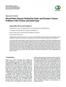
An infinite horizontal 2D duct of height h is considered. All lengths of the problem are dividedª by h, leading to a duct of unitary height D∞ = © (x1 , x2 ) ∈ R2 ; 0 < x2 < 1 of boundary ∂D∞ . The duct is filled with a compressible fluid and a part D of the duct D∞ , bounded by the vertical boundaries Σ− at x1 = 0 and Σ+ at x1 = L, is randomly filled with rigid scatterers (Fig. 1). Finally we note Ω∞ = D∞ \O the acoustic propagation domain where O is the union of the interiors of the scatterers and Γ the union of the boundaries of the scatterers. A time harmonic regime of frequency ω is considered. With time dependence e−iωt

Figure 1. Geometry

omitted, the incident pressure field is noted pinc (x) . The total pressure field P reads P = pinc + p where p is the scattered pressure satisfying the equations: ¡ ¢ ∆ + k2 p = 0 in Ω∞ ,     ∂p ∂p inc   =− on Γ, ∂n ∂n ∂p   =0 on ∂D∞ ,    P∞ ± ±iβn x1  ∂n p(x) = n=0 an e θn (x2 ) when x1 → ±∞ (radiation conditions)

(1)

where n is the exterior normal of Ω∞ and k = ωh/c is the dimensionless frequency with c the speed of sound. The radiation conditions are expressed in terms of guided modes defined in appendix A. 2.2.

Numerical method

We now present the method used to compute efficiently the scattered field. This method has three main advantages: it reduces the infinite domain Ω∞ to a finite domain Ω of small size, it selects naturally the outgoing solution and it is well-suited for a finite element approximation. 2.2.1.

Reduction to a bounded domain

Let us introduce the following integral representation of the scattered pressure field, solution of Eq. 1: ∀x = (x1 , x2 ) ∈ Ω∞ : ¶ Z µ ∂G(x, y) ∂pinc (y) p(x) = p(y) + G(x, y) dΓy , ∂ny ∂ny Γ

(2)

where y = (y1 , y2 ) and G(x, y) is the Green’s function of the medium without scatterers. The notation ∂G(x, y)/∂ny means n · ∇y G(x, y). In the free 2D space

February 22, 2010

11:15 4

Waves in Random and Complex Media

luneville˙mercier˙revised2

Eric Lun´ eville & Jean-Francois Mercier (1)

the Green’s function reads G(x, y) = H0 (k|x − y|)/4i and in the duct case it is the solution of (y ∈ D∞ is supposed fixed): ¢ ¡ 2 G(x, y) = δ(x − y) ∆ + k in D∞ , x   ∂p =0 on ∂D∞ ,  P∞ ±  ∂n ±iβ x G(x, y) = n=0 gn (y)e n 1 θn (x2 ) when x1 → ±∞. We give in appendix A the expression (modal expansion) of this Green’s function and a way to compute it. 2.2.2.

Coupling with an integral representation

Now, we present the method to reduce the computation domain. We introduce around each scatterers an artificial boundary. The union of these boundaries is noted Σ (Fig. 2) and the union of the domains between the scatterers Γ and Σ is noted Ω. It is the computation domain and it is chosen small by taking Σ close 1111111111 0000000000 0000000000 1111111111 0000000000 1111111111 Γ 0000000000 1111111111 0000000000 1111111111 0000000000 1111111111 0000000000 1111111111 0000000000 1111111111 0000000000 1111111111 Ω 0000000000 1111111111 0000000000 1111111111

Σ

1111111111 0000000000 0000000000 1111111111 0000000000 1111111111 0000000000 1111111111 Γ 0000000000 1111111111 0000000000 1111111111 0000000000 1111111111 0000000000 1111111111 Ω 0000000000 1111111111 0000000000 1111111111 0000000000 1111111111

1111111111 0000000000 0000000000 1111111111 0000000000 1111111111 0000000000 1111111111 Γ 0000000000 1111111111 0000000000 1111111111 0000000000 1111111111 0000000000 1111111111 0000000000 1111111111 Ω 0000000000 1111111111 0000000000 1111111111

Σ

Σ

Figure 2. Computational domain

to Γ. The main idea is to use the integral representation (2) to get a boundary condition on the artificial boundary Σ. For λ ∈ C, let us consider the following problem: ¡ ¢  2 p=0 ∆ + k in Ω,    ∂p ∂p  inc   =− on Γ,  µ ¶ ∂n µ ∂n ¶ Z µ ∂ ∂G(x, y) ∂ (3) + λ p(x) = +λ p(y)   ∂n ∂n ∂n  y Γ ¶    ∂pinc   + (y)G(x, y) dΓy on Σ. ∂n Problems (3) and (1) are proved to be equivalent as soon as λ ∈ C\R (see [12]). Remark 1 : If =m(λ) = 0, the problems (3) and (1) are not equivalent for the resonance frequencies k of the interior problem: ¢ (¡ ∆ + k 2 p = 0 in Ω ∪ O, ∂p = 0 on Σ. ∂n These resonance frequencies form a sequence (kn )n∈N tending to infinity. In particular when Σ is a circle of radius RΣ , they are the zeros of the first derivative 0 (kR ), m ∈ N. When =m(λ) 6= 0 and k = k , even though of Bessel functions Jm n Σ problem (3) is well-posed, some instabilities may occur in numerical computations. Better precision can be recovered by adjusting properly |=m(λ)|.

February 22, 2010

11:15

Waves in Random and Complex Media

luneville˙mercier˙revised2

Waves in Random and Complex Media

2.2.3.

5

The variational formulation

We note f = −∂pinc /∂n on Γ the©source term. The variational formulation ª R of problem (3) is: find p ∈ H 1 (Ω) = p/ Ω |p|2 + |∇p|2 < ∞ such that (Dλ = ∂ ∂nx + λ) Z Z Z Z ∂G(x, y) ∇p · ∇¯ q − k2 p¯ q + λ p¯ q− q¯(x) p(y)Dλ dΓy dΣx , ∂ny Ω Σ Σ Γ Z Z Ω Z = f q¯ − q¯(x) f (y)Dλ G(x, y) dΓy dΣx for all q ∈ H 1 (Ω).

Z

Γ

Σ

Γ

To perform numerical approximation of this formulation, a classic Lagrange finite element method is used. Let (wi )i=1,Nn be the finite element basis associated to the mesh nodes (xi )i=1,Nn . We note Pi the approximation of p(xi ), Fi = f (xi ) and we define the rigidity matrix and the mass matrices:

Kij =

Z Ω

∇wj · ∇wi and

MΛij =

Z Λ

wj wi where Λ = Ω, Σ or Γ.

Finally, we introduce the finite element interpolations of the terms involving the Green’s function: Dλ G(x, y) '

XX

NSkl wk (x)wl (y) and Dλ

k∈IΣ l∈IΓ

k∈IΣ l∈IΓ

where

XX ∂G(x, y) ' ND kl wk (x)wl (y), ∂ny

NSkl and ND kl are the single and double layer matrices: NSkl = Dλ G(xk , yl ) and ND kl = Dλ

∂ G(xk , yl ), ∂ny

where IΣ (resp. IΓ ) is the set of the indexes of the nodes located on Σ (resp. Γ). Thanks to these notations, we are lead to solve the following linear system: (K − k 2 MΩ + λMΣ − C)P = MΓ F − S, where

C = MΣ ND MΓ and S = MΣ NS MΓ F .

Remark 2 : As an alternative, an integral equation method [13] could be used with the benefit of a significant mesh size reduction (reduced to Γ). However, compared to such Boundary Element Method (BEM), the method of coupling FEM with an integral representation present the two following advantages: the numerical treatment of the singulatity of the Green’s function at x = y is avoided and it is easier to extend it to more complicated configurations: impedance boundary condition, penetrable or elastic obstacles. Besides, the maximum cost of the integral representation method lies in the evaluation of the full matrices NS and ND . Such matrices have also to be evaluated with the BEM and are nearly of the same size.

February 22, 2010

11:15

Waves in Random and Complex Media

6

2.3.

luneville˙mercier˙revised2

Eric Lun´ eville & Jean-Francois Mercier

Energy balance

To interpret the numerical results it is useful to use the energy conservation law. For any transverse section Σ of the duct, the energy flux is given by: Z µ ¯¶ ∂P ∂ P F (Σ) = P¯ −P dx2 . ∂x1 ∂x1 Σ The energy conservation law expresses as F (Σ− ) = F (Σ+ ). Thanks to the decomposition of the scattered field and total field on the guided modes of the duct (appendix A):  ∞ X    arn e−iβn x1 θn (x2 )   p(x) =      P (x) =

n=0 ∞ X

for

x1 ≤ 0, (4)

atn eiβn (x1 −L) θn (x2 )

for

x1 ≥ L,

n=0

a simple calculation, for an incident wave as the first guide mode (plane wave) with a unit amplitude pinc (x) = eikx1 , leads to: F (Σ+ ) = 2i

N X n=0

à βn |atn |2

and

F (Σ− ) = 2i k −

N X

! βn |arn |2

,

n=0

where N = [k/π] (the number of propagative modes is Np = N + 1). Therefore the energy conservation reads Finc = Ft + Fr where Finc = 2ik P t 2 is the incident energy, Ft = 2i N n=0 βn |an | the transmitted energy and Fr = PN 2i n=0 βn |arn |2 the reflected energy. An alternative writing is R + T = 1 with T = Ft /Finc and R = Fr /Finc . 2.4.

Application to the determination of an effective equivalent medium

We have chosen the following numerical procedure: the bounded part D of the duct is filled with Ns scatterers chosen as disks of radius a. We note Φ the scatterers density (or surface fraction). It is defined as the ratio of the surface occupied by the scatterers with the surface 1 × L of D: Φ = Ns πa2 /L. 2.4.1.

Mesh generation

To generate a mesh with many scatterers, we first build a reference mesh of an annular region surrounding a scatterer of radius 1 (Fig. 3 (a)), the radius of the exterior circle Σ being 1.5. The interior circle is divided in 16 points and 24 points are used for the exterior circle. A mesh made of two concentric layers of triangles is built in the annular region; it has 80 triangles and 60 vertices. The procedure to generate a finite element mesh of Ns = 50 scatterers and for L = 2 consists in dividing D in Ns square cells of size d = 1/5(= L/10), in choosing the center of the scatterers in each cell following a uniform random law (Fig. 3 (b)) and finally in scaling and translating the reference mesh according to the desired scatterers density. For a mesh of density Φ, the size of the scatterers is p a = ΦL/(Ns π). Since d is fixed, it implies that the disorder becomes weaker when the density increases. To avoid overlaping of scatterers, we prevent the exterior boundary of the reference mesh from exiting the square. This means that the scatterer center is not chosen in a square of size d but of size d − 3a. It implies

11:15

Waves in Random and Complex Media

luneville˙mercier˙revised2

Waves in Random and Complex Media

7

(a) (b) 1 0.8 0.6 0.4 0.2 0

Figure 3. (a): reference mesh

0

0.5

1

1.5

2

(b): random configuration of scatterers for Φ = 0.1

that the exclusion distance between scatterers (the minimal distance between two scatterers) is 3a and that the maximum reachable density is Φ = 0.35, obtained for a = d/3 (then the union of the scatterers and their surrounding annular regions cover (1.5)2 × 0.35 = 79% of the surface). Because of the cells subdivision, this is not a complete random realization. It is usually called a perturbed periodic scatterers array. Starting from such array, the random sequential adsorption (RSA) technique might be used to approach a complete disorder [10]. By measuring the radial distribution function (RDF) [2, 10, 14] we have measured the spatial correlation of the scatterers distribution to compare it to the underlying periodic one (Fig. 4). For the periodic case, the RFD

(2)

(a)

(1)

10

5

0

0

0.5

1 (3) 3

2

2

1

1

(b)

3

0

0

0.5

1

0

3

3

2

2

1

1

0

0.5

1

0

0.5 r

1

(c)

February 22, 2010

0

0

0.5 r

1

0

Figure 4. (a): periodic array; (b): perturbed square arrangement Φ = 0.01; (c): Φ = 0.08; (1): scatterers configurations; (2): RFD for one realization; (3): mean RFD for 500 realizations

is characterized by a peaks distribution (Fig. 4 (a)). The RFD of one realization of a perturbed square arrangement is far from this distribution (Fig. 4 (2)). This is also true after averaging on many realizations (Fig. 4 (3b)). Only for rather large densities the RFD reveals oscillations in phase with the peaks distribution of the periodic case (Fig. 4 (c)). Remark 3 : The computation time is mainly related to the computation of the

February 22, 2010

11:15

Waves in Random and Complex Media

8

luneville˙mercier˙revised2

Eric Lun´ eville & Jean-Francois Mercier

terms involving the Green’s function (evaluation of series expansion slowly converging and special treatment of singular behavior). For a configuration of 5 scatterers, the computation time is of the order of a few seconds. The computation time varies like Ns2 and the use of a complete random mesh would imply prohibitive computation times. The advantage of using a perturbed periodic array is to allow to reduce significantly the computations time: the main mesh is divided in ten meshes, each of them corresponding to one vertical slice of the main mesh. For each slice, with typically 5 scatterers, the scattering matrix is computed. Time saving results from the parallelization of the computations and from the ten times reduction of the mesh size. Finally, the scattering matrix of the main layer is obtained from the combination of the ten scattering matrices, with a neglectible computation time. 2.4.2.

Computed quantities and mean process

We note Nc the number of random configurations of scatterers taken into account to evaluate the averaged field. For j = 1 to Nc , the reflected pj and transmitted Pj pressure fields are computed in Ω using finite element approximation. The fields pj |Σ− and Pj |Σ+ are computed from the integral representation (2) and the reflect,j tion ar,j n and transmission an coefficients defined by Eq. 4 are given by: Z ar,j n =

0

Z

1

pj |Σ− θn (x2 )dx2

and

at,j n =

1

0

Pj |Σ+ θn (x2 )dx2 .

P r,j 2 For the j th pressure field, the reflected energy is Rj = N n=0 βn |an | /k and the PN t,j 2 transmited energy is Tj = n=0 βn |an | /k. They satisfy the conservation law Rj + Tj = 1 for j = 1 to Nc . The empiric mean fields are defined as: hpi(x) =

Nc ∞ X 1 X pj = harn ie−iβn x1 θn (x2 ) Nc j=1

hP i(x) =

for

Nc ∞ X 1 X Pj = hatn ieiβn (x1 −L) θn (x2 ) Nc j=1

x ≤ 0,

n=0

for

x ≥ L.

n=0

¯ = To these mean fields are associated the energies of the mean field R PN P N t 2 r 2 ¯ β |ha i| /k. These quantities are different n=0 n=0 βn |han i| /k and T = PN PNcn n r 2 from the mean energies hRi = n=0 βn h|an | i/k and hT i = j=1 Rj /Nc = PN t 2 n=0 βn h|an | i/k. Indeed, only the last ones satisfy the energy conservation hRi + hT i = 1. 2.4.3.

Models for the transmissions

The mean quantities allow to compute a numerical effective transmission Tef f = |hat0 i|2 that will be compared to transmissions given by analyticial approaches: Foldy’s and Linton-Martin’s models. They are obtained considering propagation in the free space. They indicate that the mean field is an evanescent plane wave and they link the effective wavenumber of the averaged plane wave to the incident plane wave. Foldy’s theory [3] is valid for point scatterers (at least small), far enough from each others (low surface density of scatterers, a ¿ λ ¿ d), independent and isotropic. Linton-Martin [6] have extended Foldy’s results to the anisotropic case, taking into account pair correlations and calculating the correction of order two in the surface density to Foldy’s formula: 2 kmod = k 2 + δ1 n0 + δ2 n20 + · · · ,

(5)

February 22, 2010

11:15

Waves in Random and Complex Media

luneville˙mercier˙revised2

Waves in Random and Complex Media

9

where n0 = Ns /L. This formula is derived assuming small values of the scatterer concentration (n0 a2 ¿ 1 which reads also a ¿ d) and small values of n0 /k 2 (or equivalently λ ¿ d). At the Foldy’s formula. The values of P∞first order n0 , it is the2 P P∞ ∞ the constants are δ1 = 4i n=−∞ Zn and δ2 = 4πib n=−∞ s=−∞ Zn Zs ds−n (kb) where Zn = Jn0 (ka)/Hn0 (ka), dn (x) = Jn0 (x)Hn0 (x) + [1 − (n/x)2 ]Jn (x)Hn (x) and b is the exclusion distance. In our case b = 3a. 2 To the two model wavenumbers: kF2 ol = k 2 + δ1 n0 and kLM = k 2 + δ1 n0 + δ2 n20 ik F ol L 2 we associate the transmission coefficients TF ol = |e | and TLM = |eikLM L |2 .

3.

Numerical results

In all the numerical experiments, we consider a domain of length L = 2 and Nc = 300 up to 500 configurations. The densities varies from Φ = 0.05 to 0.1 (10% of the surface covered by scatterers) and the incident wavenumber varies between k = 0.5 to 60 (dimensionless wavelength λ = 12.6 to 0.11). To deal with many parameters is one of the main difficulty of our study. In particular we have three independent distances to consider at the same time: the radius a of the scatterers, the mean distance d between scatterers and the wavelength λ of the incident wave. Once these quantities are fixed, the number Ns of scatterers (Ns d2 = L) and the density of scatterers Φ = Ns πa2 /L are deduced. For a given density there are different ways to create disorder. In order not to change many parameters at the same time to make the interpretation of results easier, we restrict to two ways of mesh generation when Φ varies: p p (1) Ns fixed: then d = p L/Ns is fixed and a = ΦL/(Ns π), (2) a fixed: then d = a π/Φ and Ns = ΦL/πa2 . The usual multiple scattering analytical models are generally established for a ¿ λ ¿ d. We always consider configurations for which a ¿ λ and a ¿ d, but we do not restrict to λ ¿ d. We consider the larger range λ/d = 0.5 to 63. In the two following subsections we fix Ns = 50 and therefore d = 0.2. 3.1.

Influence of the frequency

We consider a moderate density Φ = 0.04 which corresponds to scatterers of size a = 0.023. The frequency k varies from 0.5 to 60 which corresponds to λ/d = 0.5 to 62.8. 3.1.1.

Energy transfers

On Fig. 5 (a) is represented the mean transmitted energy hT i versus the frequency. We have observed that hRi + hT i = 1 with a good precision except the occurence of a numerical instability for the frequency k = 54.5, where a peak can also be seen on Fig. 5 (a) : this is a resonance frequency described in remark 1. The first zero of J10 (z) is in z = 1.84 leading to kres = 54.4 (RΣ = 1.5a). On Fig. 5 (a) is seen that for small frequencies the mean transmitted energy hT i ' 1: the wavelength is so long that the scatterers are “transparent” and all the injected energy is transmitted. For large frequencies, scattering effects are strong and most of the mean energy is reflected (hRi = 1−hT i ' 0.7 for k = 60). On Fig. 5 (b) we get that ¯ + T¯ < 1 because of the loss of energy the total energy of the mean field satisfies R through the averaging process. More precisely hT i measures the transmitted energy of the whole field while T¯ measures the transmitted energy of the coherent field. Thus hT i − T¯ measures the transmitted energy of the incoherent field. Excepting

11:15

Waves in Random and Complex Media

10

luneville˙mercier˙revised2

Eric Lun´ eville & Jean-Francois Mercier (a)

(b)

1

1

0.9 0.8

0.8

0.6 ¯ T¯ R,



0.7 0.6

0.4

0.5 0.4

0.2

0.3 0.2

0

20

40

0

60

0

20

k

40

60

k

¯ dot: R ¯ + T¯ Figure 5. Φ = 0.04; (a): hT i versus k; (b): solid line: T¯, dashdot: R,

around the frequencies k = 15.5 and k = 30.5 (see explanations latter) we obtain ¯ ' 0 which indicates that the mean field is essentially transmitted. R To go further, we have determined how the energy is distributed over the modes of the duct. The reflected and transmitted the guided P energy can be decomposedr on 2 i/k. This is modes: for example one gets hRi = N hRi where hRi = β h|a | n n n n n=0 the mean reflected energy carried by the nth propagative mode. We have found that the mean reflected energy is carried by all the propagative modes whereas the mean transmitted energy is mainly carried by the plane mode. In a same way, only ¯'R ¯ 0 = |har i|2 and the plane mode is involved in the energy of the mean field: R 0 t 2 ¯ ¯ T ' T0 = |ha0 i| . In other words, the mean field is a plane wave, as assumed in theoretical models. The peaks observed on Fig. 5 (a) and (b) at k = 15.5 and k = 30.5 correspond to some of the band gap frequencies of the “underlying” periodic array (Ns = 50 scatterers located at the middle on the square cells). Band gap frequencies of the (a)

(b) 1

0.8

0.8

0.6

0.6

periodic

1

R

Tperiodic

February 22, 2010

0.4

0.2

0

0.4

0.2

0

10

20

30 k

40

50

60

0

0

10

20

30 k

40

50

60

Figure 6. (a) Transmission and (b) reflection (solid line :mode 0, dot : mode 10) in a periodic array

periodic array are shown on Fig. 6: they correspond to a drop of the transmission or a maximum of the reflection when sending a plane wave on the periodic array. Only modes 0, 10, 20, · · · can be produced by an incident plane wave. Indeed, due to some properties of the the geometry and of the data, both symmetrical about the midline y = 1/2 and vertically periodic with 5 periodicity cells, we can prove by constructing explicit solutions and by a uniqueness argument that the scattered field expands only on the modes of orders n = 2 × 5 × p, p ∈ N. Of course this argument fails once disorder is introduced. On Fig. 6 (b) are represented separately the reflections of mode 0 (solid line) and of mode 10 (doted line). Mode 10 becomes

11:15

Waves in Random and Complex Media

luneville˙mercier˙revised2

Waves in Random and Complex Media

11

propagative for k ≥ 31.5 (10π = 31.4) and mode 20 for k ≥ 60. Modes 0 and 10 behave differently and two kind of band gaps exist. First the ones associated with a strong reflection of the mode 0 (k = 15.5, 30.5 and 47). They correspond respectively to λ = 2d, d and 2d/3. Therefore they agree with the law kd = nπ, n integer, for a one-dimensional periodic array [15]. This law is usually no longer valid in a 2D periodic array [15] and thus seems to extend to 2D arrays in ducts for plane mode propagation. The other band gap family corresponds to a strong reflection of the mode 10 (k = 40 and 52). On Fig. 5 (b), only the low frequency band gaps of the plane mode k = 15.5 and 30.5 are seen. We do not observe any drop behavior of T¯ at the larger band gap frequencies k = 40, 47 and 52, but notice that T¯ is too small to be clearly interpreted above k = 31.5. It could have been expected that an averaged perturbed periodic array would behave like a periodic array. Comparison of the transmission in the perturbed (Fig. 5 (b)) and unperturbed periodic array (Fig. 6 (a)) contradicts this expectation. For the frequencies outside the fondamental band gaps, T¯ and Tperiodic are completly different and, as we will see latter, only T¯ obeys a multiple-scattering law. On the contrary, for frequencies in the fondamental band gaps below the cut-off of the 10th guided mode, we recover the behavior of the periodic array. The influence of the periodic band gaps would probably disappear in case of complete randomness as suggested by [10] in the case of one realization. 3.1.2.

Effective transmissions (a) Φ=0.04

(b) Φ=0.08 1

0.8

0.8

0.6

0.6 T

1

T

February 22, 2010

0.4

0.4

0.2

0.2

0

0

10

20

30 k

40

50

60

0

0

10

20

30 k

40

50

60

Figure 7. solid line: numerical values, dot: Foldy, dash: LM

On Fig. 7 (a) the numerical transmission is compared to the theoretical transmissions versus the frequency. Good accordance is found excepting for the band gap frequencies k = 15.5 and 30.5. It is not possible to decide which model, Foldy or LM, is closer from numerical experiments. On Fig. 7 (b) are represented the same quantities for a larger density Φ = 0.08. As expected, the numerical values go away from the model ones when the density increases. Moreover the drops of the numerical transmission at the band gap frequencies are amplified, because the perturbation of the periodic array is less random for larger densities. Note that LM model seems to be more suited than Foldy’s model for low frequencies.

3.2.

Influence of the density

Now, the frequency k is fixed and we study the influence of the density Φ = 0 to 0.1 which corresponds to scatterers sizes a = 0.008 to 0.036. We have studied the case of an incident wave with λ varying from 3d to d/2 (Fig. 8). A general observation

11:15

Waves in Random and Complex Media

12

luneville˙mercier˙revised2

Eric Lun´ eville & Jean-Francois Mercier

is that for all frequencies, the difference between Tef f and Tmod (mod = F ol or LM ) is very small for small densities. (a) k=10

(b) k=15

0.9

0.8

0.8

0.6 T

1

T

1

0.7

0.4

0.6

0.2

0.5

0

0.02

0.04

Φ

0.06

0.08

0

0.1

0

0.02

(c) k=20

0.04

Φ

0.06

0.08

0.1

0.08

0.1

(d) k=60

1

0.8

0.8

0.6 T

0.6 T

February 22, 2010

0.4

0.4 0.2

0.2 0

0

0.02

0.04

Φ

0.06

0.08

0.1

0

0

0.02

0.04

Φ

0.06

Figure 8. Φ = 0.04; solid line: numerical values, dot: Foldy, dash: LM

In the case k = 10 (λ = 3d) is found that the attenuation in a duct is weaker than the attenuation predicted by models derived in the free space. It is due to the guided effect of the duct. Foldy’s model predicts to much attenuation and TLM is the closest from Tef f . For the case k = 15 (λ = 2d), agreement between numerical and theoretical results is very poor. As already mentioned, this is because we are close from a band gap frequency of the periodic array and it is not a multiple scattering regime. At last, for small wavelengths k = 20 to k = 60 (then λ = d/2), Fig. 8 shows good accordance between numerical effective wavenumber and theoretical models developed in the free space. This means that in a duct guided effects are weaker than multiple-scattering effects.

3.3.

Other configurations

Finally, in this section, we consider other ways to create random configurations: by reducing the mean distance d, by increasing the number of scatterers Ns or by changing the scatterers shape. 3.3.1.

Case d = 0.1

We have studied the influence of halving the mean distance d : 0.2 → 0.1. Then the scatterers size is reduced a → a/2 and the number of scatterers increases Ns → 4Ns = 200 (20 × 10 scatterers). In the free space, multiple scattering is invariant by scaling: when all the distances of the problem, d, λ and a, are halved, the multiple scattering effects are the same. In particular for the models wavenumbers, applying the scaling k → 2k (since λ → λ/2) in Eq. 5 leads to kmod → 2kmod (and thus kmod d constant). Therefore in the free space, the two pertinent nondimensional parameters are the density Φ = π(a/d)2 and d/λ (or kd). The numerical experiments (for d = 0.1 and k = 20, k = 30 and k = 40) in a duct show the same behavior. In other words, the number of scatterers in a vertical section of the duct does not influence significantly the values of the effective parameters.

February 22, 2010

11:15

Waves in Random and Complex Media

luneville˙mercier˙revised2

Waves in Random and Complex Media

3.3.2.

13

Case of a fixed scatterers size

p When the size of the scatterers a = 0.01 is fixed (d = a π/Φ varies from 0.25 to 0.05) we can still assume we are mostly in the regime a ¿ d. The number of scatterers Ns varies in a large range from 32 to 648 and for large values of Ns time computations become very long. Fig. 9 shows an example of arrangement and the associated RFD for Φ = 0.04 (Ns = 23 × 11 = 253). One advantage to work with (b) (a)

(c)

2

2

1.5

1.5

1

1

0.5

0.5

0

0

0.5 r

0

1

0

0.5 r

1

Figure 9. (a): perturbed square arrangement for Φ = 0.04; (b): RFD for one realization; (3): mean RFD for 500 realizations

a fixed size of scatterers is that the step of the mesh, and thus the finite element error, is fixed when k or φ vary. The conclusion is the same than in the previous paragraph: the values of the effective transmission just depends pon the value of kd. The results obtained for a frequency k and a distance d = a π/Φ are the same than the results associated to d0 = 0.2 (for instance) and a frequency k 0 such that kd = k 0 d0 . 3.3.3.

Extension to square scatterers

Our numerical method extends naturally to any scatterers shape, for example squares. Only the reference mesh has to be changed and it is represented on Fig. 10 (a). To a random location in each cell, a random rotation is applied to the squares (see an example on Fig. 10 (b)). From the curve of the transmission versus the (a)

(b) 1 0.8 0.6 0.4 0.2 0

0

0.5

1

1.5

2

Figure 10. (a): reference mesh, (b): example of a random configuration

frequency for Φ = 0.08 (Fig. 11), we observe behaviors similar to those for circular scatterers. In particular at the band gap frequencies the transmission vanishes. Tef f is farther from Tmod than in the disks case (same density), but such models have been developed for circular obstacles. After the second band gap at k = 30.5, Tef f nearly vanishes whereas it was small for disks configuration because of stronger scattering effect of squares corners.

4.

Conclusion

We have developed a numerical approach to determine the effective properties of a random medium in a duct. The choice of a FEM method allows to consider

11:15

Waves in Random and Complex Media

14

luneville˙mercier˙revised2

Eric Lun´ eville & Jean-Francois Mercier

1 0.9 0.8 0.7 0.6 T

February 22, 2010

0.5 0.4 0.3 0.2 0.1 0

0

10

20

30 k

40

50

60

Figure 11. Φ = 0.08; solid line: numerical values, dot: Foldy, dash: LM

scatterers of arbitrary shapes whereas the coupling of FEM with an integral representation, based on the duct Green’s function, allows to reduce significantly the mesh size. Time saving is also obtained by considering a perturbed periodic array for the scatterers positions instead of complete randomness: the scatterers are placed on a reference periodic array and are moved locally randomly. We have shown that the effective medium is well described by analytical models, Foldy’s and Linton-Martin models, although they are not designed for a duct configuration, except for the lowest band gap frequencies of the reference periodic array. In that case, the effective medium behaves like a periodic one. Appendix A. Green’s function of a guide

It is convenient to define the Green’s function of the duct thanks to the duct mode i.e. the solution p(x1 , x2 ) of Helmholtz equation in the duct with Neuman boundary condition on the rigid walls and with separated variables p(x1 , x2 ) = θ(x2 )eiβx1 . The transverse modes read for all n ∈ N: p θn (x2 ) = 2 − δn0 cos (nπx2 ) and define an orthonormal basis of L2 (]0, 1[). The wavenumbers βn are given by: q βn =

k 2 − (nπ)2

if

n≤

k π

and

q βn = i (nπ)2 − k 2

if

n>

k . π

A real βn corresponds to a propagative mode and an evanescent mode is associated to a complexe βn . It is straightforward to determine the Green’s function of the duct as a modal expansion [16]: G(x, y) =

∞ iβn |x1 −y1 | X e n=0

2iβn

θn (x2 )θn (y2 ).

(A1)

Note that the Green’s function is not defined if there exists n such that βn = 0. This happens for the sequence of the cut-off frequencies of the duct k ∈ {kn = nπ, n ∈ N}. In practice we avoid these frequencies. It is convenient to write the Green’s function as ∞

G(x, y) =

eiβn |x1 −y1 | eik|x1 −y1 | X + Gn where Gn = cos (nπx2 ) cos (nπy2 ) . 2ik iβn n=1

February 22, 2010

11:15

Waves in Random and Complex Media

luneville˙mercier˙revised2

REFERENCES

15

As Gn has the following asymptotic behavior: Gn

− n→∞ ∼

e−nπ|x1 −y1 | cos (nπx2 ) cos (nπy2 ) , nπ

the expansion (A1) is semi-convergent when |x1 − y1 | = 0 and converges slowly when |x1 − y1 | is small (weak exponential decay). A classicalPway [16] to recover a ˜ = ∞ Gn : fast convergent series is to extract the singular part of G n=1 S(x, y) = −

∞ −nπ|x1 −y1 | X e n=1

nπ

cos (nπx2 ) cos (nπy2 ) .

This expansion S is still semi-convergent but has an exact analytical expression: n 1 S(x, y) = ln 4e−2π|x1 −y1 | [cosh (π|x1 − y1 |) − cos (π(x2 + y2 ))] , 4π × [cosh (π|x1 − y1 |) − cos (π(x2 − y2 ))]} . Finally we define the “residual” part which has a better convergence: ˜ y) − S(x, y) = R(x, y) = G(x,

∞ X n=1

Ã

eiβn |x1 −y1 | e−nπ|x1 −y1 | + iβn nπ

! cos (nπy2 ) ,

such that G = (eik|x1 −y1 | /2ik) + S + R. When |x1 − y1 | = 0, the terms of the expansion behave like n−3 . Thanks to this fast convergence, only a few term in the sum are necessary to get a good approximation of the Green’s function. In practice the number of term taken into acount is chosen such that the error is less than 1%. References [1] M. Chekroun, L. Le Marrec, B. Lombard, J. Piraux and O. Abraham, Comparison between a multiple scattering method and direct numerical simulations for elastic wave propagation in concrete, Ultrasonic Wave Propagation in Non Homogeneous Media, Series: Springer Proceedings in Physics, 128 (2008), A. Leger, M. Deschamps (Eds.) pp. 317–327. [2] A. Derode, V. Mamou, A. Tourin, Influence of correlations between scatterers on the attenuation of the coherent wave in a random medium, Phys. Rev. E 74 (2006), id. 036606. [3] L.L. Foldy, The multiple scattering of waves. I: General Theory of isotropic scattering by randomly distributed scatterers. Physical Review. 67 (1945), pp. 107–119. [4] V. Twersky, On Scattering of Waves by Random Distributions. I. Free-Space Scatterer Formalism, J. Math. Phys. 3 (1962), pp. 700–715. [5] B.C. Gupta and Z. Ye, Localization of classical waves in two-dimensional random media: A comparison between the analytic theory and exact numerical simulation, Physical Review E 67 (2003), id. 036606. [6] C.M. Linton and P.A. Martin, Multiple scattering by random configurations of circular cylinders: Second-order corrections for the effective wavenumber, J. Accoust. Soc. America 117 (2005), pp. 3413–3423. [7] K. Nakashima, S. Biwa and E. Matsumoto, Elastic Wave Transmission and Stop Band Characteristics in Unidirectional Composites, J Journal of Solid Mechanics and Materials Engineering 2 (2008), pp. 1195–1206. [8] J. Segurado and J. Llorca, A numerical approximation to the elastic properties of sphere-reinforced composites, Journal of the Mechanics and Physics of Solids 50 (2002), pp. 2107–2121. [9] N.A. Gumerov and R. Duraiswami, Computation of scattering from clusters of spheres using the fast multipole method, J. Acoust. Soc. Am. 117 (2005), pp. 1744–1761. [10] S. Biwa, F. Kobayashi and N. Ohno, Influence of disordered fiber arrangement on SH wave transmission in unidirectional composites, Mechanics of Materials 39 (2007), pp. 1–10. [11] R.-B. Yang and A.K. Mal, Multiple scattering of elastic waves in a fiber-reinforced composite, J. Mech. Phys. Solids 42 (1994), pp. 1945–1968. [12] A. Jami and M. Lenoir, A variational formulation for exterior problems in linear hydrodynamics, Comput. Method Appl. Mech. Engrg. 16 (1978), pp. 341–359. [13] W.L. Wendland, Boundary Element Topics, Springer (1995).

February 22, 2010

11:15 16

Waves in Random and Complex Media

luneville˙mercier˙revised2

REFERENCES

[14] R. Pyrz, Correlation of microstructure variability and local stress field in two-phase materials, Mater. Sci. Eng. A177 (1994), pp. 253-259. [15] F. Kobayashi, S. Biwa and N. Ohno, Wave transmission characteristics in periodic media of finite length: multilayers and fiber arrays, Int. J. Solids Struct. 41 (2004), pp. 7361–7375. [16] R.E. Collin, Field theory of guided waves, IEEE Press (1991), pp. 78–86.