Research Article Maximum Likelihood Sequence Detection Receivers ...

Hindawi Publishing Corporation Journal of Electrical and Computer Engineering Volume 2015, Article ID 736267, 12 pages http://dx.doi.org/10.1155/2015/736267

Research Article Maximum Likelihood Sequence Detection Receivers for Nonlinear Optical Channels Gabriel N. Maggio,1 Mario R. Hueda,1 and Oscar E. Agazzi2 1

Laboratorio de Comunicaciones Digitales, Universidad Nacional de Córdoba, CONICET, Avenida Vélez Sarsfield 1611, Córdoba X5016GCA, Argentina 2 ClariPhy Communications, Inc., 7585 Irvine Center Drive, Suite 100, Irvine, CA 92618, USA Correspondence should be addressed to Gabriel N. Maggio; [email protected] Received 25 July 2014; Revised 12 November 2014; Accepted 14 January 2015 Academic Editor: Martin Haardt Copyright © 2015 Gabriel N. Maggio et al. This is an open access article distributed under the Creative Commons Attribution License, which permits unrestricted use, distribution, and reproduction in any medium, provided the original work is properly cited. The space-time whitened matched filter (ST-WMF) maximum likelihood sequence detection (MLSD) architecture has been recently proposed (Maggio et al., 2014). Its objective is reducing implementation complexity in transmissions over nonlinear dispersive channels. The ST-WMF-MLSD receiver (i) drastically reduces the number of states of the Viterbi decoder (VD) and (ii) offers a smooth trade-off between performance and complexity. In this work the ST-WMF-MLSD receiver is investigated in detail. We show that the space compression of the nonlinear channel is an instrumental property of the ST-WMF-MLSD which results in a major reduction of the implementation complexity in intensity modulation and direct detection (IM/DD) fiber optic systems. Moreover, we assess the performance of ST-WMF-MLSD in IM/DD optical systems with chromatic dispersion (CD) and polarization mode dispersion (PMD). Numerical results for a 10 Gb/s, 700 km, and IM/DD fiber-optic link with 50 ps differential group delay (DGD) show that the number of states of the VD in ST-WMF-MLSD can be reduced ∼4 times compared to an oversampled MLSD. Finally, we analyze the impact of the imperfect channel estimation on the performance of the ST-WMF-MLSD. Our results show that the performance degradation caused by channel estimation inaccuracies is low and similar to that achieved by existing MLSD schemes (∼0.2 dB).

1. Introduction Maximum likelihood sequence detection (MLSD) receivers for nonlinear channels have been extensively investigated in the literature (e.g., [1, 2] and references therein). Their ability to achieve optimal performance in the presence of additive white Gaussian noise (AWGN) has always been of great theoretical and practical interest. The theoretical interest lies in that it provides a performance bound for any reception scheme. The practical interest stems from its ability to actually achieve optimal or nearly optimal performance in transmissions over nonlinear channels. Much of the early work in this area has been focused on the compensation of nonlinearities in satellite communications [1–5]. A traditional architecture for the optimal nonlinear receiver consists of a matched-filter bank (MFB) followed by a maximum likelihood sequence detector (MLSD) [1].

Owing to the correlation among the spatial noise components at the MFB outputs, an MLSD with non-Euclidean metrics must be used. The use of oversampling in combination with MLSD (OS-MLSD) has also been proposed to implement the optimal receiver in the presence of nonlinearities (see [2] and references therein). Since the complexity of both MFB and OS MLSD-based receivers grows exponentially with the channel memory, their practical application in transmissions over highly dispersive channels has been limited. Despite this fact, MLSD-based receivers are still preferred over decision feedback equalizers (DFE) in applications such as multigigabit intensity modulation/direct detection (IM/DD) fiber optic systems for the two following reasons. (i) Performance: DFE suffers from severe performance limitations in moderate to high dispersion singlemode fiber links as a result of its inability to compensate nonlinear ISI [6, 7]. Although nonlinear

2

Journal of Electrical and Computer Engineering DFE (NL-DFE) structures have also been considered in the literature (e.g., [8, 9]), their performances still degrade significantly at long fiber lengths (e.g., ≥500 km). On the other hand, MLSD can operate with a constant penalty around 3 dB with respect to backto-back (B2B) at virtually any distance [10, 11]. (ii) High-speed implementation: future generation of communication systems will operate at multigigabit per second data rates on highly dispersive channels [12]. In commercial applications, the digital receiver is often implemented as a monolithic chip in CMOS technology [12]. Maximum clock frequency of stateof-the-art complex digital signal processors in 28 nm CMOS technology is limited to frequencies lower than ∼1 GHz. Therefore, in order to achieve multigigabit per second data rates, parallel processing techniques are required [12]. Although the complexity of serial implementations of DFE grows linearly with channel memory, all presently known parallel processing implementations require that the bottleneck created by the feedback loop be broken using techniques such as the ones proposed by [13–15], whose complexity grows exponentially with the channel memory. Therefore, in high-speed applications, complexity of both DFE and MLSD increases with the channel memory in a similar way.

From the above it is clear that complexity reduction of MLSD is crucial for many practical applications. In IM/DD optical channels, the receiver must compensate the linear fiber dispersion as well as nonlinearities caused by lasers, optical modulators, the fiber Kerr effect, photo-detectors, and other components of the link. Chromatic dispersion (CD) and polarization-mode dispersion (PMD), in combination with the quadratic response of the photo-detector, are major factors that limit the reach and drive the complexity of optical-transmission systems at data rates ≥10 Gb/s [16, 17]. With traditional implementations based on oversampling techniques, an 8192-state MLSD is required to compensate 700 km of fiber at 10 Gb/s [10]. This is prohibitive in current CMOS technology1 . A new MLSD receiver architecture for nonlinear channels has been proposed in [18]. The major breakthrough of this proposal consists in a novel representation of the received signal obtained by a Gram-Schmidt-like orthogonalization of the kernels of a Volterra series expansion of the channel. This procedure yields a special form of space-time whitened matched filter (ST-WMF) [19] whose baud-rate-sampled outputs are sufficient statistics with independent noise components in both space and time. Combined with the minimum phase property of the response of each branch, the ST-WMF provides an effective way to reduce the complexity of MLSD in nonlinear channels. The ST-WMF MLSD technique offers a smooth trade-off between performance and complexity. As complexity is progressively reduced, performance degrades in a graceful manner. Numerical results in [18] demonstrate that the number of states of the VD in ST-WMF-MLSD required on a 10 Gb/s, 700 km, and IM/DD fiber-optic link

without PMD can be reduced 8 times compared to an oversampled MLSD. Further contributions on the ST-WMF-MLSD receiver and its performance on IM/DD optical links are provided in this work. First, the space channel compression achieved by the ST-WMF-MLSD is analyzed in detail. Space channel compression is important because it is the property that enables the major complexity reductions of the proposed architecture. Second, the performance evaluation of the STWMF-MLSD receiver is extended by addressing the combined effect of CD and PMD. Numerical results confirm that the ST-WMF-MLSD remains an attractive solution in the presence of these combined impairments. Finally, the impact of channel estimation inaccuracies on the ST-WMFMLSD performance is assessed. Accuracy and speed of channel estimation are particularly important when tracking nonstationary channels. Nonstationarity in optical channels results from PMD and random rotations of the laser state of polarization. Our results show that the performance degradation caused by an imperfect channel estimation is low and similar to that achieved by existing MLSD schemes (∼0.2 dB). This paper is organized as follows. The nonlinear channel model and the ST-WMF-MLSD architecture are described in Sections 2 and 3, respectively. Performance evaluation of the ST-WMF-MLSD under different channel conditions, as well as its robustness in the presence of imperfect channel knowledge, are presented and discussed in Sections 4 and 5. Finally, conclusions are drawn in Section 6.

2. Nonlinear Channel Model The noisy received signal is given by 𝑟 (𝑡) = 𝑠 (𝑡) + 𝑧 (𝑡) ,

(1)

where 𝑠(𝑡) is the noise-free signal and 𝑧(𝑡) is the noise component, which is assumed to be a white Gaussian process with power spectral density 𝑁0 . Component 𝑠(𝑡) can be expressed in terms of its Volterra-series expansion [20, 21]. For example, neglecting the DC term of the expansion we get 𝑁−1

𝑠 (𝑡) = ∑𝑎𝑘 𝑓0 (𝑡 − 𝑘𝑇) + ∑ ∑𝑎𝑘 𝑎𝑘−𝑚 𝑓𝑚 (𝑡 − 𝑘𝑇) , 𝑘

(2)

𝑚=1 𝑘

where 𝑓0 (𝑡) is the linear kernel, 𝑓𝑚 (𝑡) with 𝑚 > 0 is the 𝑚th second-order kernel, 𝑎𝑘 is the 𝑘th symbol at the input of the nonlinear channel, 1/𝑇 is the symbol rate, and 𝑁 is the total number of kernels2 . 2.1. Channel Model Orthogonalization. Next we present an alternative representation of the nonlinear signal 𝑠(𝑡) [18]. Without loss of generality, we consider here the Volterraseries with a dominant linear kernel 𝑓0 (𝑡), and we select the first pivoting response as ℎ0 (𝑡) = 𝑓0 (𝑡). Let H0 be the signal space spanned by the set {ℎ0 (𝑡 − 𝑘𝑇)} [19]. We assume that signal spaces are Hilbert spaces with inner product defined ∞ as ∫−∞ 𝑥(𝑡)𝑦∗ (𝑡) 𝑑𝑡, where superscript ∗ denotes complex

Journal of Electrical and Computer Engineering

3

conjugate. From the projection theorem, the nonlinear kernels 𝑓𝑚 (𝑡) can be uniquely expressed as (0) ℎ0 (𝑡 − 𝑛𝑇) + 𝑔𝑚 𝑓𝑚 (𝑡) = ∑𝜆(0,𝑚) (𝑡) , 𝑛

Thus, note that 𝑠1 (𝑡) is orthogonal to the signal spaces H0 and H1 , spanned by {ℎ0 (𝑡 − 𝑘𝑇)} and {ℎ1 (𝑡 − 𝑘𝑇)}, respectively. Repeating the processing on (11) and generalizing, we get

(3)

𝑛

(0) where 𝑔𝑚 (𝑡) is orthogonal to the signal space H0 ; that is,

∫

∞

−∞

(0) 𝑔𝑚 (𝑡) ℎ0∗ (𝑡 − 𝑗𝑇) 𝑑𝑡 = 0,

𝑚 = 1, . . . , 𝑁 − 1, ∀𝑗 ∈ Z,

(0) while ∫−∞ |𝑔𝑚 (𝑡)|2 𝑑𝑡 is minimum [19], and Z denotes the set of all integers. We highlight that the first summation in (3) is the projection of 𝑓𝑚 (𝑡) onto H0 . Define G0𝑚 as the signal space (0) spanned by {𝑔𝑚 (𝑡−𝑘𝑇)}. For 𝑥(𝑡) ∈ H0 and 𝑦(𝑡) ∈ G0𝑚 , from ∞ (4) note that ∫−∞ 𝑥(𝑡)𝑦∗ (𝑡) 𝑑𝑡 = 0; therefore 𝑥(𝑡) and 𝑦(𝑡) are orthogonal signals [19]. Replacing (3) in (2) and operating, we obtain

(5)

𝑁−1

(6)

𝑚=1

(7)

𝑘 𝑚=1

with operator ⊗ denoting convolution. Notice that 𝑠0 (𝑡) ∈ H0 0 and 𝑠0 (𝑡) ∈ ∪𝑁−1 𝑚=1 G𝑚 ; therefore signals 𝑠0 (𝑡) and 𝑠0 (𝑡) are orthogonal (see (4)). Next we focus on 𝑠0 (𝑡). Without loss of generality we select the second pivoting response as ℎ1 (𝑡) = 𝑔1(0) (𝑡); then (7) can be rewritten as 𝑁−1

(0) 𝑠0 (𝑡) = ∑𝑎𝑘 [𝑎𝑘−1 ℎ1 (𝑡 − 𝑘𝑇) + ∑ 𝑎𝑘−𝑚 𝑔𝑚 (𝑡 − 𝑘𝑇)] . 𝑚=2

(8) Similarly to (5)–(7), 𝑠0 (𝑡) can be expressed as 𝑠0 (𝑡) = 𝑠1 (𝑡) + 𝑠1 (𝑡) ,

(9)

where 𝑁−1

𝑠1 (𝑡) = ∑ [𝑎𝑘 𝑎𝑘−1 + ∑ 𝑎𝑘 𝑎𝑘−𝑚 ⊗ 𝜆(1,𝑚) ] ℎ1 (𝑡 − 𝑘𝑇) , (10) 𝑘 𝑚=2

𝑁−1

(1) 𝑠1 (𝑡) = ∑ ∑ 𝑎𝑘 𝑎𝑘−𝑚 𝑔𝑚 (𝑡 − 𝑘𝑇) ,

(11)

𝑘 𝑚=2

chosen to satisfy with 𝜆(1,𝑚) 𝑛 ∫

∞

−∞

(1) 𝑔𝑚 (𝑡) ℎ1∗ (𝑡 − 𝑗𝑇) 𝑑𝑡 = 0,

for 𝑚 = 2, . . . , 𝑁 − 1, ∀𝑗 ∈ Z.

(12)

(13)

if 𝑛 = 0 if 0 < 𝑛 < 𝑁 − 1 if 𝑛 = 𝑁 − 1, (14)

with ∫

∞

ℎ𝑚 (𝑡) ℎ𝑛∗ (𝑡 − 𝑗𝑇) 𝑑𝑡 = 0 𝑚 ≠ 𝑛, ∀𝑗 ∈ Z.

(15)

From (13) and (15) note that signal components from different paths are orthogonal; that is, ∞

−∞

(0) 𝑠0 (𝑡) = ∑ ∑ 𝑎𝑘 𝑎𝑘−𝑚 𝑔𝑚 (𝑡 − 𝑘𝑇) ,

𝑘

𝑏𝑘(𝑛)

∫

𝑁−1

𝑘

𝑛=0 𝑘

{ { 𝑎𝑘 + ∑ 𝑎𝑘 𝑎𝑘−𝑚 ⊗ 𝜆(0,𝑚) { 𝑘 { { { 𝑚=1 { 𝑁−1 ={ { 𝑎𝑘 𝑎𝑘−𝑛 + ∑ 𝑎𝑘 𝑎𝑘−𝑚 ⊗ 𝜆(𝑛,𝑚) { 𝑘 { { 𝑚=𝑛+1 { { {𝑎𝑘 𝑎𝑘−𝑁+1

−∞

where

𝑘

𝑛=0

𝑁−1

∞

] ℎ0 (𝑡 − 𝑘𝑇) , 𝑠0 (𝑡) = ∑ [𝑎𝑘 + ∑ 𝑎𝑘 𝑎𝑘−𝑚 ⊗ 𝜆(0,𝑚) 𝑘

𝑁−1

where ℎ𝑛 (𝑡) is the response of the 𝑛th channel path and with 𝑏𝑘(𝑛) given by

(4)

𝑠 (𝑡) = 𝑠0 (𝑡) + 𝑠0 (𝑡) ,

𝑁−1

𝑠 (𝑡) = ∑ 𝑠𝑛 (𝑡) = ∑ ∑𝑏𝑘(𝑛) ℎ𝑛 (𝑡 − 𝑘𝑇) ,

𝑠𝑚 (𝑡) 𝑠𝑛∗ (𝑡) 𝑑𝑡 = 0,

𝑚 ≠ 𝑛.

(16)

Figure 1 shows two multiple input-single output (MISO) representations of the nonlinear channel. Figure 1(a) shows the signal represented by the traditional Volterra model of (2); Figure 1(b) depicts the orthogonal representation given by (13) and (14). 2.2. Space Channel Compression. The model orthogonalization procedure described in Section 2.1 can be performed in 𝑁! different ways with 𝑁 being the number of kernels. For example, consider a Volterra model with 𝑁 = 3. One way to obtain the orthogonalized model may be realized by selecting the kernels as shown in Figure 2. In this case, the pulse 𝑓0 (𝑡) is selected as the pivoting ℎ0 (𝑡) for the first orthogonalization step. Then, 𝑔1(0) and 𝑔2(0) are obtained as the components of 𝑓1 (𝑡) and 𝑓2 (𝑡) orthogonal to ℎ0 (𝑡) = 𝑓0 (𝑡). For the second step, 𝑔1(0) (𝑡) is selected as the pivoting response, so 𝑔2(1) (𝑡) results as the component of 𝑔2(0) (𝑡) orthogonal to ℎ1 (𝑡) = 𝑔1(0) (𝑡). This unique ordering could be identified by the following set of indexes I = {0, 1, 2}. A different result is achieved by selecting the pivoting responses as illustrated in Figure 3. In this situation, 𝑓1 (𝑡) is selected as the pivoting response for the first step, and 𝑔1(0) (𝑡) and 𝑔2(0) (𝑡) are the components of 𝑓0 (𝑡) and 𝑓2 (𝑡) orthogonal to ℎ0 (𝑡) = 𝑓1 (𝑡). According to Figure 3, 𝑔2(0) (𝑡) (which is different from 𝑔2(0) (𝑡) shown in Figure 2) is selected as the pivoting response for the second orthogonalization step. Then, 𝑔2(1) (𝑡) will be obtained as the component of 𝑔1(0) (𝑡) orthogonal to ℎ1 (𝑡) = 𝑔2(0) (𝑡). The index set corresponding to the procedure depicted in Figure 3 is I = {1, 2, 0}.

4


ak

ak

bk(0)

ak ak−1 .. . ak ak−N+1

bk(1)

f0 (t)

ak ak−1 .. .

ak ak−N+1

f1 (t) .. .

s(t)

+

fN−1 (t)

h0 (t) h1 (t) .. .

Mapping

bk(N−1)

(a)

hN−1 (t)

s0 (t) s1 (t) +

s(t)

sN−1 (t)

(b)

Figure 1: MISO model of the nonlinear channel: (a) based on a Volterra representation; (b) based on the spatially compressed orthogonal representation.

f0 (t) selected as the pivot for 1st step:

ak f0 (t)

ak ak−1 f1 (t)

ak ak−2 f2 (t)

ak

𝜆(0,1) k

𝜆(0,2) k

1st orthogonalization step: g1(0) (t)

h0 (t)

selected as the pivot for 2nd step:

2nd orthogonalization step:

bk(0) = ak + ak ak−1 ⊗ 𝜆(0,1) + ak ak−2 ⊗ 𝜆(0,2) k k

bk(1) = ak ak−1 + ak ak−2 ⊗ 𝜆(1,2) k bk(2)

g1(0) (t)

g2(0) (t)

ak ak−1

𝜆(1,2) k

h1 (t) (Trivial step):

= ak ak−2

g2(1) (t) ak ak−2

f1 (t) selected as the pivot for 1st step:

1st orthogonalization step: selected as the pivot for 2nd step:

ak f0 (t)

ak ak−1 f1 (t)

ak ak−2

ak ak−1

𝜆(0,1) k

𝜆(0,2) k

h0 (t)

2nd orthogonalization step:

bk(0) = ak ak−1 + ak ⊗ 𝜆(0,1) + ak ak−2 ⊗ 𝜆(0,2) k k bk(1) = ak ak−2 + ak ⊗ 𝜆(1,2) k bk(2) = ak

f2 (t)

g1(0) (t)

g2(0) (t)

ak ak−2

𝜆(1,2) k

h1 (t)

g2(1) (t)

𝑃−1

𝑖=0

𝑖=0

̂ ≠ Iop , ∀I

(17)

󵄨󵄨 (𝑖) 󵄨󵄨2 ∞ 󵄨󵄨 󵄨󵄨𝑏𝑘 󵄨󵄨 } ∫ 󵄨󵄨ℎ𝑖 (𝑡)󵄨󵄨󵄨󵄨2 𝑑𝑡 = 𝐸 { E(𝑖) I 󵄨 󵄨 −∞

(18)

where

is the energy in the 𝑖th path for the set I, while 𝐸{⋅} denotes expectation. If 𝑃 = 𝑁, notice that any orthogonalization process I will satisfy condition (17). Otherwise, if 𝑃 < 𝑁 the criterion guarantees that the signal energy contained in the complete 𝑃 paths shall be maximum, independent of the individual energy distribution among them. The optimum channel expansion that satisfies (17) can be found by an exhaustive search. Instead, we propose to achieve the orthogonalization process to meet the following criteria: ̂ (1) ≥ ⋅ ⋅ ⋅ ≥ E ̂ (𝑁−1) , ̂ (0) ≥ E E

(Trivial step): ak h2 (t)

Figure 3: Orthogonalization procedure following the ordering I = {1, 2, 0}.

Note that the set of responses {ℎ𝑖 (𝑡)}2𝑖=0 and sequences resulting from the procedures described in Figures 2 and 3 are two different expansions of the same signal 𝑠(𝑡). Any one of the 𝑁! possible sets can be selected in the orthogonalization process. Space compression of the channel can be achieved concentrating the maximum of the channel energy on a reduced set of paths, independent of the distribution of their individual energy, as explained in the following discussion. Let 𝑃 be a given number of paths used to model the channel (e.g., if 𝑃 = 𝑁, note that any orthogonalization process {𝑏𝑘(𝑖) }2𝑖=0

𝑃−1

(𝑖) ∑ E(𝑖) Iop ≥ ∑ EI ̂,

h2 (t)

Figure 2: Orthogonalization procedure following the ordering I = {0, 1, 2}.

g2(0) (t)

I shall represent exactly the behavior of the channel). To reduce the complexity of the receiver, it is desirable for 𝑃 to be as small as possible. On the other hand, to minimize the performance degradation (or the inaccuracy of the channel representation), the orthogonalization process should be carried out in such a way that the most part of the signal energy is concentrated on these 𝑃 paths. From the above, for a given value of 𝑃, the optimum set Iop for space compression (i.e., minimal channel distortion modeling) should meet the following condition:

∞

(19)

̂ (𝑗) = ∫ |ℎ𝑛 (𝑡)|2 𝑑𝑡. Condition (19) can be achieved with E −∞ by selecting at each orthogonalization step (𝑖th step, e.g., with 𝑖 ∈ {1, 2, . . . , 𝑁}) the pivoting response (ℎ𝑖−1 (𝑡)) as the response with highest energy among the remaining responses (those orthogonal to ∩𝑖−2 𝑛=0 H𝑛 for 𝑡 = 𝑘𝑇, ∀𝑘). That is, at the first step we select the pivoting response ℎ0 (𝑡) as the Volterra kernel with the highest energy in {𝑓𝑛 (𝑡)}𝑁−1 𝑛=0 . At the second step we select the pivoting response ℎ1 (𝑡) as the response with highest energy in the set of responses orthogonal to H0 (0) (i.e., 𝑔𝑚 (𝑡), with 𝑚 = 1, 2, . . . , 𝑁 − 1). This procedure is repeated in the same way at each step, where the best pivoting response at each stage is selected by an exhaustive search among all the pivot candidates at that stage. The minimization of the energy of the orthogonal responses (see (3), (4), and associated discussion) ensures that condition (19) is met. As we shall show later, condition (19) gives rise to space channel compression, which can be exploited to reduce complexity.


𝑓𝑚 (𝑡) are orthogonal (same) pulses ∀𝑚). Thus, we conclude the following for the channel analyzed in the example.

L = 700 km

0 Normalized cumulative path energy (dB)

5

−0.05

(i) Most energy of the nonlinear kernels with the traditional Volterra model is contained in their projection onto the linear signal space spanned by the set {ℎ0 (𝑡 − 𝑘𝑇)} = {𝑓0 (𝑡 − 𝑘𝑇)}.

−0.1 −0.15 −0.2

(ii) A channel model with 2 paths captures practically all the signal energy.

−0.25 −0.3 −0.35

0

1

2

3 4 Path index, n

5

6

7

Traditional Volterra representation Orthogonalized Volterra representation

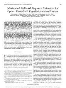
Figure 4: Normalized cumulative path energy of the nonlinear IM/DD fiber-optic link with 𝐿 = 700 km and 1/𝑇 = 10 Gb/s.

2.3. Example. As an example, we present results for a 10 Gb/s, 700 km, and IM/DD fiber-optic link (details about the simulated system are given in Section 4.1). Without loss of generality, we assume that 𝑎𝑘 ∈ {±1}. Let S𝑛 be the normalized cumulative path energy of the traditional Volterra-series expansion (see (2)) given by 𝑛

∞

1 󵄨2 󵄨 S𝑛 = ∑ ∫ 󵄨󵄨󵄨𝑓𝑚 (𝑡)󵄨󵄨󵄨 𝑑𝑡, 𝐸𝑠 𝑚=0 −∞

𝑛 = 1, 2, . . . , 𝑁 − 1,

(iii) Since E(0) I is ∼97.5% of the total signal energy (see Figure 4). Therefore, as we shall show later, a receiver that considers the first channel path should be able to achieve a good performance.

3. MLSD Receiver for Nonlinear Channels with AWGN The MLSD receiver chooses the sequence {𝑎𝑘 } that minimizes the metric 𝐽=∫

𝑁−1 𝑚=0

𝑛

1 S𝑛 = ∑ E(𝑚) , 𝐸𝑠 𝑚=1 I

𝑛 = 0, 1, . . . , 𝑁 − 1,

𝑁−1

∞

𝑛=0

−∞

𝐽 ∝ −2 ∑ R {∑𝑏𝑘(𝑛) ∫

(20)

𝑁−1

𝑘

𝑛=0

∞

where E(𝑚) I is given by (18) with I obtained according to the criteria defined by (19). In all cases, note that S𝑛 ≤ 1 ∀𝑛, with S𝑁−1 = 1. Figure 4 shows the normalized cumulative path energy S𝑛 for the traditional (20) and orthogonalized (22) Volterraseries representation with 𝑁 = 8. For the orthogonal representation, the pivoting responses are selected according to the criteria in (19). We observe that most energy of the nonlinear signal is concentrated on the first two paths for (1) the orthogonalized Volterra-series expansion (i.e., E(0) I + EI represents ∼99.4% of the total signal energy). The traditional Volterra model requires five paths to capture a similar level of nonlinear signal energy. We highlight that the increase of S𝑛 from −0.33 dB to −0.12 dB at 𝑛 = 0 is due to the factor 𝐸{|𝑏𝑘(0) |2 } ≥ 1 in (18). Notice that this factor is a measure of the correlation between all nonlinear kernels 𝑓𝑚 (𝑡) with 𝑚 > 0 and the linear kernel 𝑓0 (𝑡) (e.g., 𝐸{|𝑏𝑘(0) |2 } = 1 (𝑁) if 𝑓0 (𝑡) and

(24)

𝑁−1

𝑁−1

∞

𝑛=0

−∞

= −2 ∑ R {∑𝑏𝑘(𝑛) 𝑟(𝑛) 𝑘 }+ ∑ ∫ 𝑛=0

(22)

𝑟 (𝑡) ℎ𝑛∗ (𝑡 − 𝑘𝑇) 𝑑𝑡}

󵄨2 󵄨󵄨 󵄨󵄨𝑠𝑛 (𝑡)󵄨󵄨󵄨 𝑑𝑡 −∞

+ ∑∫

(21)

On the other hand, the normalized cumulative path energy of the orthogonalized Volterra-series expansion is defined as

(23)

Using (13) and (16) in (23), we get

∞

󵄨2 󵄨󵄨 󵄨󵄨𝑓𝑚 (𝑡)󵄨󵄨󵄨 𝑑𝑡. −∞

|𝑟(𝑡) − 𝑠(𝑡)|2 𝑑𝑡.

−∞

where 𝐸𝑠 is the total energy of the signal component 𝑠(𝑡): 𝐸𝑠 = ∑ ∫

∞

𝑘

󵄨2 󵄨󵄨 󵄨󵄨𝑠𝑛 (𝑡)󵄨󵄨󵄨 𝑑𝑡,

where R denotes the real part, while 𝑟(𝑛) 𝑘 =∫

∞

−∞

𝑟 (𝑡) ℎ𝑛∗ (𝑡 − 𝑘𝑇) 𝑑𝑡,

𝑛 = 0, 1, . . . , 𝑁 − 1. (25)

From (24) notice that the computation of the cost function 𝐽 for every candidate symbol sequence {𝑎𝑘 } can be achieved from the samples at the outputs of the matched filters given by (25). From (1), equation (25) can be rewritten as (𝑛) (𝑛) 𝑟(𝑛) 𝑘 = 𝑠𝑘 + 𝑧𝑘 ,

𝑛 = 0, 1, . . . , 𝑁 − 1,

(26)

where 𝑠(𝑛) 𝑘 =∫

∞

−∞

𝑧(𝑛) 𝑘

=∫

∞

−∞

𝑠 (𝑡) ℎ𝑛∗ (𝑡 − 𝑘𝑇) 𝑑𝑡, (27) 𝑧 (𝑡) ℎ𝑛∗

(𝑡 − 𝑘𝑇) 𝑑𝑡.

(𝑚) ∗ From (15) note that 𝐸{𝑠(𝑛) 𝑙 [𝑠𝑙−𝑘 ] } = 0 if 𝑚 ≠ 𝑛 while

𝑁0 𝜌𝑘(𝑛) , if 𝑛 = 𝑚 (𝑚) ∗ 𝐸 {𝑧(𝑛) [𝑧 ] } = { 𝑙 𝑙−𝑘 0, otherwise,

(28)

6

Journal of Electrical and Computer Engineering where Φ(𝑡) and M𝑘 are 𝑁 × 𝑁 diagonal matrices given by

where 𝜌𝑘(𝑛) = ∫

∞

−∞

ℎ𝑛 (𝑡) ℎ𝑛∗ (𝑡 − 𝑘𝑇) 𝑑𝑡.

(29)

Since the noise is assumed Gaussian, from (28) we conclude that the noise components at the output of the proposed MFB are spatially independent. Therefore, the bank of matched filters {ℎ𝑛∗ (−𝑡)}𝑁−1 𝑛=0 followed by a baud rate sampler is called the space-whitened matched filter (S-WMF) bank. 3.1. Space-Time Whitened Matched Filter MLSD Receiver. From the above, we observed that the matched filter bank derived from the new expansion of the nonlinear channel gives rise to spatially independent noise components. In order to simplify the implementation of the sequence detector, a space and time whitening filter bank is derived. Let 𝜙𝑛 (𝑡) be the impulse response of the filter with Fourier transform (FT) given by 𝐻 (𝜔) Φ𝑛 (𝜔) = (𝑛) 𝑛 𝑗𝜔𝑇 , 𝛾 𝑀𝑛 (𝑒 )

𝑛 = 0, . . . , 𝑁 − 1,

(30)

(𝑛)

where 𝐻𝑛 (𝜔) is the FT of ℎ𝑛 (𝑡) and 𝛾 and 𝑀𝑛 (𝑧) are defined by the folded spectrum factorization 𝑆𝑛 (𝑧) = (𝛾(𝑛) )2 𝑀𝑛 (𝑧)𝑀𝑛∗ (1/𝑧∗ ) with 𝑆𝑛 (𝑧) being the 𝑍-transform of the sequence 𝜌𝑘(𝑛) given by (29). The set {𝜙𝑛 (𝑡 − 𝑘𝑇)} forms an orthonormal basis for the signal space spanned by {ℎ𝑛 (𝑡 − 𝑘𝑇)}. Furthermore, we choose 𝑀𝑛 (𝑧) to be minimum phase [19]. Define 𝑟̃𝑛 (𝑡) as the projection of 𝑟(𝑡) onto the signal space spanned by {ℎ𝑛 (𝑡 − 𝑘𝑇)}; that is, 𝑟̃𝑛 (𝑡) = ∑𝑟̃𝑘(𝑛) 𝜙𝑛 (𝑡 − 𝑘𝑇) ,

(31)

𝑘

∞

where 𝑟̃𝑘(𝑛) = ∫−∞ 𝑟(𝑡)𝜙𝑛∗ (𝑡 − 𝑘𝑇) 𝑑𝑡. From (15) and following the procedure used in [19, Section 10.2.4], metric (23) can be expressed as 󵄩󵄩 󵄩󵄩2 󵄩󵄩 󵄩󵄩 󵄩 𝐽 = ∫ 󵄩󵄩̃r(𝑡) − ∑H(𝑡 − 𝑘𝑇)b𝑘 󵄩󵄩󵄩 𝑑𝑡, 󵄩 󵄩󵄩 −∞ 󵄩 𝑘 󵄩 󵄩 ∞

(32)

where H(𝑡) is an 𝑁 × 𝑁 diagonal matrix given by ℎ0 (𝑡) 0 0 ℎ1 (𝑡) H (𝑡) = ( . .. .. . 0 0

⋅⋅⋅ ⋅⋅⋅

0 0 .. .

d ⋅ ⋅ ⋅ ℎ𝑁−1 (𝑡)

),

(33)

while 𝑇

b𝑘 = [𝑏𝑘(0) 𝑏𝑘(1) ⋅ ⋅ ⋅ 𝑏𝑘(𝑁−1) ] ,

(34) 𝑇

̃r (𝑡) = [̃𝑟0 (𝑡) 𝑟̃1 (𝑡) ⋅ ⋅ ⋅ 𝑟̃𝑁−1 (𝑡)] ,

(35)

with 𝑏𝑘(𝑛) and 𝑟̃𝑛 (𝑡) given by (14) and (31), respectively. On the other hand, from (30) it is possible to show that ∑H (𝑡 − 𝑘𝑇) b𝑘 = ∑Φ (𝑡 − 𝑘𝑇) [M𝑘 ⊗ b𝑘 ] , 𝑘

𝑘

(36)

𝜙0 (𝑡) 0 0 𝜙1 (𝑡) Φ (𝑡) = ( . .. .. . 0 0 𝛾(0) 𝑚𝑘(0) M𝑘 = (

0 .. .

0

𝛾

⋅⋅⋅ ⋅⋅⋅

0 0 .. .

0

⋅⋅⋅

0

𝑚𝑘(1)

⋅⋅⋅

0 .. .

(1)

.. .

d

0

),

(37)

d ⋅ ⋅ ⋅ 𝜙𝑁−1 (𝑡)

),

(38)

⋅ ⋅ ⋅ 𝛾(𝑁−1) 𝑚𝑘(𝑁−1)

with 𝑚𝑘(𝑛) being the inverse FT of 𝑀𝑛 (𝑒𝑗𝜔𝑇 ). From (31) notice that (35) can be expressed as ̃r (𝑡) = ∑Φ (𝑡 − 𝑘𝑇) ̃r𝑘 , 𝑘

(39)

where ̃r𝑘 = [̃𝑟𝑘(0) ⋅ ⋅ ⋅ 𝑟̃𝑘(𝑁−1) ]𝑇 (see (31)). From (32), (36), and (39) it can be shown that MLSD reduces to minimize 󵄩2 󵄩 𝐽 = 󵄩󵄩󵄩̃r𝑘 − M𝑘 ⊗ b𝑘 󵄩󵄩󵄩 .

(40)

Let ̃z𝑘 be the 𝑁-dimensional vector with the noise components of the baud rate samples ̃r𝑘 . From (15) and (30), the power spectral density of ̃z𝑘 results in S𝑧̃ = 𝑁0 I, where I is the identity matrix. Therefore, the minimization of (40) can be easily implemented by using a Viterbi detector with multidimensional Euclidean branch metrics. Figure 5 shows a block diagram of the ST-WMF-MLSD receiver with dimension 𝑃 (i.e., 𝑃 is the number of filters in the bank). If 𝑃 = 𝑁, all the paths of the nonlinear channel are used by the receiver. 3.2. Complexity Considerations. The ST-WMF-MLSD consists of a filter bank followed by a Viterbi decoder (VD) and a channel estimation stage. Although the computational load of the latter may be important, its complexity is not critical since it can be implemented at a low frequency rate3 . On the other hand, the dimension of the front-end (𝑃) is expected to be very low in general as a result of the spatial energy compression achieved by the ST-WMF-MLSD. Then, 𝑃 ≤ 2 is a reasonably good estimation for applications in IM/DD optical systems and the computational complexity of the filter bank is reduced to the one of 2 linear filters. Therefore, the implementation complexity of ST-WMF-MLSD is dominated by the VD. Practical aspects related to highspeed implementations of VD have been widely investigated in the past literature (e.g., see [12, 22] for more details). The computational load (usually measured in number of multiplications and comparisons) and storage requirements of the VD depend directly on the number of states. Therefore, we adopt the number of states of the VD as the measure of complexity in order to compare the MLSD architectures investigated in this work.


r(0) (t)

H0∗ (𝜔)

r(t)

7 kT

r(0) k

r(1) k

r(1) (t)

H1∗ (𝜔) .. .

.. . r(P−1) k

r(P−1) (t)

∗ HP−1 (𝜔)

̃r(0) k

1 𝛾(0) M0∗ (ej𝜔T )

̃r(1) k

1 𝛾(1) M1∗ (ej𝜔T )

VD

.. .

â k

̃r(P−1) k

1 ∗ (ej𝜔T ) 𝛾(P−1) MP−1

Figure 5: Block diagram of the 𝑃-dimensional ST-WMF-MLSD receiver. ASE noise Photodetector ak

MOD

Optical fiber

Nonlinear transf. √(·)

+ Optical filter

r(t)

ST-WMF MLSD

â k

Electrical filter

Figure 6: IM/DD fiber-optic system with ST-WMF-MLSD receiver.

4. Performance Evaluation in IM/DD Optical Systems Next we analyze the proposed ST-WMF-MLSD receiver in transmissions over IM/DD fiber-optic systems with on-off keying (OOK) modulation. We focus on two key aspects of ST-WMF-MLSD: its performance (in comparison with current solutions based on OS-MLSD), and its ability to reduce complexity (e.g., number of states of VD). Complexity reduction is possible owing to (i) the minimum-phase property of the equivalent channel response provided by STWMF and (ii) condition (19). The latter gives rise to space compression, which reduces the ST-WMF dimension, 𝑃. This is achieved by using the most significant 𝑃 paths of the nonlinear channel. Figure 6 depicts the optical system under consideration. The transmitter modulates the intensity of the transmitted signal using NRZ-OOK modulation. The standard single mode fiber (SMF) introduces CD and PMD, as well as attenuation. Optical amplifiers are deployed periodically along the fiber to compensate the attenuation, also introducing amplified spontaneous emission (ASE) noise in the signal. ASE noise is modeled as AWGN in the optical domain. The received optical signal is filtered by an optical filter and then converted to a current with a PIN diode or avalanche photodetector. The resulting photocurrent is filtered by an electrical filter. The noise component after the electrical filtering is non-Gaussian and signal-dependent [16]. Therefore, the electrical signal is first processed by a memoryless nonlinear transformation. It has been found that after a square root transformation, the noise can be assumed Gaussian and signal-independent [23, 24]. Furthermore, channel nonlinearities can also be reduced by using the square root transformation [25], which improves the space compression used to reduce the receiver dimension (i.e., most

of the channel energy is concentrated on the linear kernel). The split-step Fourier method [26] is used to compute the propagation of optical signals through the fiber. Oversampled linear and nonlinear kernels are extracted from the electrical signal after the square root transformation. The oversampling factor 𝑅 = 𝑇/𝑇𝑠 depends on various parameters of the communication system (e.g., optical power, fiber length, etc.). In our case, we have found that an oversampling factor of 𝑅 = 16 is good enough to accurately model the system; that is, no improvement was appreciated by increasing the sampling rate for the entire set of conditions considered for according this work. Then, we compute ℎ𝑛 (𝑘𝑇𝑠 ) and 𝜆(𝑛,𝑚) 𝑘 to (17), and the symbol rate channel response matrix M𝑘 can be easily obtained from (38). Since the noise after the square root transformation is approximately Gaussian and signal-independent [27], the theory proposed in [28] is used to evaluate the bit error probability4 . All the kernels of the nonlinear channel are used to compute the error probability, independent of the receiver dimension, 𝑃. Data rate is 1/𝑇 = 10 Gb/s and the transmitted pulse shape has an unchirped 2 2 Gaussian envelope 𝑒−𝑡 /2𝑇0 with 𝑇0 = 36 ps. We use a Lorentzian optical filter and a fourth-pole Butterworth electrical filter with bandwidths of 15 and 10 GHz, respectively. The fiber dispersion is 𝐷 = 17 ps/(nm-km). 4.1. IM/DD Systems with CD and PMD. Typically, the performance of equalization stages in fiber optic transmissions is evaluated by using the optical signal-to-noise ratio (OSNR) required to achieve a given BER (e.g., see [10, 11]). The target BER is around 10−3 , which corresponds to the value required at the input of the forward error correction (FEC) code to achieve the error rate expected by the application (e.g., ∼ 10−15 ) [29].

Journal of Electrical and Computer Engineering OSNR penalty @ BER = 10−3 (dB)

8 8 7.5 7 6.5 6 5.5 5 4.5 4 3.5 3

5. Impact of the Imperfect Channel Knowledge

6

8

10

12

14

16

18

log 2 (number of states)

ST-WMF-MLSD (P = 1 filter) OS-MLSD (2 samples/bit)

MLSD bound

Figure 7: OSNR penalty with respect to B2B at BER = 10−3 versus number of states of the VD for 𝐿 = 700 km and DGD = 0 ps.

Performance evaluation of the ST-WMF-MLSD has been achieved by assuming a perfect knowledge of the channel. In the following, we analyze the impact of the channel estimation inaccuracy on the performance of the ST-WMF-MLSD architecture in transmissions over IM/DD optical systems. This study will show that the performance degradation in STWMF-MLSD receivers, with 𝑃 = 1, caused by an imperfect channel estimation, is low (∼0.2 dB) and similar to that achieved by oversampled OS-MLSD receivers in the 𝐿 = 700 km fiber link used in the example of Figure 7. The estimation of the oversampled linear and nonlinear kernels is required to implement both MLSD-based receivers. Let 𝑅 = 𝑇/𝑇𝑠 be the oversampling factor. Based on the polyphase filter representation of the oversampled channel response (see Figure 9), the received samples can be expressed as 𝑁−1

𝑟𝑛(𝑖) = ∑𝑎𝑘 𝑓0(𝑖) [𝑛 − 𝑘] + ∑ ∑ 𝑎𝑘 𝑎𝑘−𝑚 𝑓𝑚(𝑖) [𝑛 − 𝑘] + 𝑧𝑛(𝑖) , (41) Figure 7 depicts the OSNR penalty with respect to a B2B system at a bit-error rate (BER) of 10−3 versus the number of states of the VD for 𝐿 = 700 km. We present results for STWMF-MLSD with 𝑃 = 1 (i.e., only one filter in the bank). For OS-MLSD with 2 samples/bit, the reduction of states is achieved by truncation and optimization of the sampling phase in order to minimize BER (8 uniformly distributed phases in the interval 𝑇/2 were tested). From Figure 7, we verify that the number of states of the VD at a penalty of 4.6 dB can be reduced from 2048 to 256 with ST-WMF-MLSD and 𝑃 = 1. Notice that this performance is achieved by using a VD with one sample per bit [11]. Furthermore, we emphasize that these benefits greatly outperform the extra complexity required by the linear filter and the channel estimator (implementation details are omitted here due to space limitations). From Figure 7 we can also see that the performance degradation achieved with 𝑃 = 1 with respect to the ideal MLSD is only ∼0.3 dB. This result can be understood from the analysis of Section 2.2, where it has been observed that 97.5% of the total signal energy is contained in the first channel path. The performance of ST-WMF-MLSD in the presence of CD and first-order PMD (i.e., differential group delay or DGD) is investigated. Figure 8 depicts the OSNR penalty versus the number of states of the VD for a 700 km fiber link with two values of DGD: 25 and 50 ps. We evaluate the OSMLSD with 2 samples/bit and ST-WMF-MLSD with 𝑃 = 2. As expected, both receivers tend to the same performance as the number of states of the VD increases. We also note that the benefits of the ST-WMF-MLSD reduce when the DGD increases5 . Nevertheless, from Figure 8 notice that the number of states of the VD at a penalty of 6 dB can be reduced 8 and 4 times with ST-WMF-MLSD at 25 and 50 ps DGD, respectively. These results show that the ST-WMFMLSD is still an attractive solution to reduce complexity in transmissions over fiber-optic channels in the presence of PMD.

𝑘 𝑚=1

𝑘

where 𝑟𝑛(𝑖) = 𝑟(𝑛𝑇 + 𝑖𝑇𝑠 ), 𝑧𝑛(𝑖) = 𝑧(𝑛𝑇 + 𝑖𝑇𝑠 ), and 𝑓𝑚(𝑖) [𝑛] = 𝑓𝑚 (𝑛𝑇 + 𝑖𝑇𝑠 ) with 𝑖 = 0, . . . , 𝑅 − 1. Notice that there are 𝑅 different sequences sampled at the baud rate, corresponding to 𝑅 different sampling phases. Equation (41) can be rewritten as 𝑁−1

𝑟𝑛(𝑖) = ∑𝑎𝑛−𝑘 𝑓0(𝑖) [𝑘] + ∑ ∑ 𝑎𝑛−𝑘 𝑎𝑛−𝑘−𝑚 𝑓𝑚(𝑖) [𝑘] + 𝑧𝑛(𝑖) . (42) 𝑘 𝑚=1

𝑘

Since symbols 𝑎𝑘 are assumed zero-mean and i.i.d. real random variables with 𝜎𝑎2 = 𝐸{|𝑎𝑘 |2 }, we can verify that 𝑓0(𝑖) [𝑘] = 𝑓𝑚(𝑖) [𝑘] =

1 𝐸 {𝑟𝑛(𝑖) 𝑎𝑛−𝑘 } , 𝜎𝑎2

1 𝐸 {𝑟𝑛(𝑖) 𝑎𝑛−𝑘 𝑎𝑛−𝑘−𝑚 } , 𝜎𝑎4

(43)

𝑖 = 0, . . . , 𝑅 − 1. From (43), a simple estimator of the oversampled linear and nonlinear kernels can be implemented with an averaging filter as follows: 𝑓̂0(𝑖) [𝑘] =

𝑛 +𝐿 −1

1 0 𝐴 (𝑖) ∑ 𝑟 𝑎̂ , 2 𝜎𝑎 𝐿 𝐴 𝑛=𝑛0 𝑛 𝑛−𝑘 𝑛 +𝐿 −1

(44)

1 0 𝐴 (𝑖) 𝑓̂𝑚(𝑖) [𝑘] = 4 , ∑ 𝑟 𝑎̂ 𝑎̂ 𝜎𝑎 𝐿 𝐴 𝑛=𝑛0 𝑛 𝑛−𝑘 𝑛−𝑘−𝑚 where 𝐿 𝐴 is the length of the averaging filter, 𝑛0 is an arbitrary time index, and 𝑎̂𝑘 is the detected symbol6 . The accuracy of the channel estimation given by (44) depends on the precision of the decisions 𝑎̂𝑘 , the length of the averaging filter 𝐿 𝐴 , and the channel noise power. We consider that decisions provided by the forward error correction (FEC) decoder are available; therefore the effect of decision errors can be

Journal of Electrical and Computer Engineering DGD = 25 ps

8 7.5

7.5

7

7

6.5 6 5.5 5 4.5

6.5 6 5.5 5 4.5

4

4

3.5

3.5

3

6

8

10

12

DGD = 50 ps

8

OSNR penalty @ BER = 10−3 (dB)

OSNR penalty @ BER = 10−3 (dB)

9

14

16

18

3

6

8


ST-WMF-MLSD (P = 2) OS-MLSD (2 samples/bit)

10 12 14 log 2 (number of states)

ST-WMF-MLSD (P = 2) OS-MLSD (2 samples/bit)

MLSD bound

(a)

16

18

MLSD bound

(b)

Figure 8: OSNR penalty respect to B2B at BER = 10−3 versus number of states of the VD for 𝐿 = 700 km. DGD = 25 ps (a) and 50 ps (b). 1/T f0(0) [n]

ak

f0(1) [n]

sn(1)

sn(0) , sn(1) , . . . , sn(R−1) s(t) = ∑ ak f0 (t − kT)

.. .

f0(R−1) [n]

1/Ts

sn(0)

k

sn(R−1)

sn(i) = s(nT + iTs ) = ∑ k ak f0(i) [n − k] f0(i) [n] = f0 (nT + iTs ) i = 0, 1, . . . , R − 1

Figure 9: Example of the polyphase filter representation of an oversampled linear channel with 𝑅 = 𝑇/𝑇𝑠 .

neglected (i.e., 𝑎̂𝑘 = 𝑎𝑘 ). We highlight that this assumption is still valid if pre-FEC decisions are used as a result of the low bit error rates experienced in this link (e.g., ∼10−3 ). From the above, we conclude that the goodness of the estimates (44) shall mainly depend on the filter length 𝐿 𝐴 and the channel noise power. The precision of (44) improves as the value of 𝐿 𝐴 increases. On the other hand, the maximum value of 𝐿 𝐴 shall be imposed by the speed of temporal variations of the fiber optic channel. As a result of its dependence on stress and vibrations, as well as on random changes in the state of polarization of the laser, PMD is nonstationary. Fluctuations with a time scale of a hundreds of microseconds have been considered in previous works (e.g., [30]). Therefore, the

response time of channel estimation algorithms for PMD mitigation must be less than 1 ms (in practice a response time less than 100 𝜇s is required [27]). This imposes, for example, that the bandwidth of the averaging filter (∼1/(4𝐿 𝐴 𝑇)) should be ≥20 kHz in order to efficiently track the channel variation. The received signal seen by an MLSD receiver in the presence of imperfect knowledge of the channel dispersion can be expressed as 𝑁−1

𝑟̃𝑛(𝑖) = ∑𝑎𝑛−𝑘 (𝑓0(𝑖) [𝑘] + ∑ 𝑎𝑛−𝑘−𝑚 𝑓𝑚(𝑖) [𝑘]) 𝑚=1

𝑘

+

𝑧𝑛(𝑖)

+

𝑧̂𝑛(𝑖)

= 𝑠𝑛(𝑖) + 𝑧𝑛(𝑖) + 𝑧̂𝑛(𝑖) ,

(45)

Journal of Electrical and Computer Engineering 2.2

2.2

2

2

1.8

1.8

1.6

1.6

SNR penalty, ΔSNR (dB)

SNR penalty, ΔSNR (dB)

10

1.4 1.2 1 0.8

1.4 1.2 1 0.8

0.6

0.6

0.4

0.4

0.2

0

0.5

1 Filter length, L A

1.5

2

×105

0.2 104

105 Averaging filter BW (Hz)

(a)

106

(b)

ΔSNR =

(46)

where 𝜎𝑧2 is the channel noise power required to achieve a BER = 10−3 with an unconstrained complexity OS-MLSD receiver (i.e., the VD uses as many states as required) and 𝜎𝑧̂2 is the variance of the estimation error component7 . Notice that the penalty is ∼0.4 dB for 𝐿 𝐴 = 105 . This value of 𝐿 𝐴 represents a BW of ∼1/(4𝐿 𝐴𝑇) = 25 kHz (see Figure 10(b)). Assuming that the estimation error is white Gaussian noise with power 𝜎𝑧̂2 , from Figure 10(a) we infer that the SNR penalty caused by an imperfect channel knowledge in OSMLSD receivers with 𝐿 𝐴 = 105 should be ≲ΔSNR ∼ 0.4 dB. Figure 11 depicts the OSNR penalty at BER = 10−3 versus the number of states of the Viterbi detector (VD) with 𝐿 = 700 km. We present results with perfect knowledge of the fiber dispersion (denoted as 𝐿 𝐴 = ∞), and for imperfect channel estimation with 𝐿 𝐴 = 105 . We see that the mean penalty caused by inaccuracies of channel estimation agrees with that expected from Figure 10 with 𝐿 𝐴 = 105 (i.e., ∼0.14 dB < ΔSNR ∼ 0.4 dB). Furthermore, we observe that the impact of imperfect channel knowledge on the

OSNR penalty @ BER = 10

𝜎𝑧2 + 𝜎𝑧̂2 , 𝜎𝑧2

−3

where 𝑠𝑛(𝑖) = 𝑠(𝑛𝑇 + 𝑖𝑇𝑠 ) and 𝑧̂𝑛(𝑖) = 𝑠̂(𝑛𝑇 + 𝑖𝑇𝑠 ) − 𝑠(𝑛𝑇 + 𝑖𝑇𝑠 ) is the estimation error component, while 𝑠̂(𝑛𝑇 + 𝑖𝑇𝑠 ) is the synthesized signal obtained from (44). Figure 10(a) shows the SNR penalty caused by the imperfect channel estimation as a function of 𝐿 𝐴 obtained from computer simulations. We consider 1/𝑇 = 10 GHz, 𝑅 = 16, and the fiber link with 𝐿 = 700 km, as used in Figure 7. The SNR penalty caused by an imperfect channel estimation is computed as

(dB)

Figure 10: SNR penalty caused by imperfect channel estimation versus length of the averaging filter (a) and the bandwidth of the averaging filter (b).

8 7.5 7 6.5 6 5.5 5 4.5 4 3.5 3

6

8

10

12

14

16

18


ST-WMF-MLSD (P = 1 filter) − L A = ∞ ST-WMF-MLSD (P = 1 filter) − L A = 105 OS-MLSD (2 samples/bit) − L A = ∞ OS-MLSD (2 samples/bit) − L A = 105 MLSD bound − L A = ∞

Figure 11: OSNR penalty at BER = 10−3 versus number of states of the VD with 𝐿 = 700 km.

performance is similar in both MLSD receivers (i.e., ∼0.14 dB and ∼0.18 dB for OS and ST-WMF, resp.). This result can be understood from the fact that the filters ℎ0∗ (−𝑡) and 𝑚𝑘(0) are computed from the samples of the estimated linear kernel 𝑓̂0 (𝑡). Taking into account that the energy of the linear component is significantly higher than the nonlinear kernels [25] (see Section 2.2), an accurate estimation of ℎ0 (𝑡) can be achieved for the channel considered. Then, we infer that the ̂0 (𝑡) energy loss of the signal component at the output of 𝑚 will be small. Therefore, and based on (45), notice that the

Journal of Electrical and Computer Engineering performance of OS-MLSD and ST-WMF-MLSD with 𝑃 = 1 should degrade in a similar way.

6. Conclusions New results on the recently proposed ST-WMF-MLSD nonlinear receiver have been presented in this paper. These results are the following: (1) the space compression property of the factorization introduced in [18] has been analyzed in detail; (2) the performance of the ST-WMF-MLSD in IM/DD fiber optic systems in the combined presence of CD and PMD has been evaluated, and (3) it has been shown that the performance degradation caused by an imperfect channel estimation and tracking is low and similar to that achieved by existing MLSD schemes. These features make the ST-WMFMLSD a good architecture for receivers for long distance IM/DD fiber-optic links.

Conflict of Interests The authors declare that there is no conflict of interests regarding the publication of this paper.

Acknowledgment This paper has been supported in part by Fundación Fulgor and the ANPCyT (PICT 2013, no. 2724).

Endnotes 1. Some commercial implementations of VD at 10 Gb/s with 4, 8, and 16 states are available in 90 nm CMOS technology [31–33]. It should be possible to implement VD’s with 64 or 128 states by using the available 28 nm technology. 2. The Volterra model can be easily extended to include higher order terms (e.g., third order kernels 𝑓𝑚 (𝑡), with input sequence 𝑎𝑘 𝑎𝑘−𝑚 𝑎𝑘−𝑛 and 𝑛 > 0, could be included in the expansion). To keep the notation simple, only second order kernels are used in the derivations throughout this paper. However, numerical results incorporate nonlinear kernels of order higher than two. 3. As a result of its dependence on stress and vibrations, as well as on random changes in the state of polarization of the laser, PMD is nonstationary. Fluctuations with a time scale of a few milliseconds have been observed in PMD measurements [27]. Thus, the response time of the channel estimation schemes for PMD mitigation must be less than 1 ms. In practice, a response time less than 100 𝜇s is required. Therefore, the channel estimation stage could be easily implemented by using current technology. 4. We did not run Monte Carlo simulations of the communication systems. The numerical results are semianalytic, in the sense that they are theoretic estimations assisted by numerical simulations. The probability of error is

11 estimated according to the theory proposed in [28]; that is, the first terms of the union bound (those with the lowest distance) are used to estimate the probability of error. Numerical simulations are used to find the distances of the error-events, their Hamming weights, and a priori probabilities. These results are then introduced in the formulas for the probability of error estimation as reported in [28]. 5. In order to explain this result, consider a fiber channel with DGD = 100 ps only (i.e., no CD). Since DGD ∼ 𝑇, the IM/DD system approximately behaves as a duobinary channel; therefore the time compression achieved by the ST-WMF-MLSD will be negligible. 6. In order to improve the channel tracking capability, an efficient implementation of the channel estimator with the well-known LMS algorithm may be preferred [12]. Nevertheless, the objective is to shed light on the impact of imperfect knowledge of the fiber dispersion on the orthogonalized Volterra model. Therefore, practical aspects of the receiver architecture (e.g., buffers, number of taps of the WF, finite precision arithmetic effects, etc.) are not considered. 7. The mean penalty of 20 runs with different seeds of the random number generator is presented.

References [1] S. Benedetto and E. Biglieri, Principles of Digital Transmission with Wireless Applications, Kluwer Academic, 1999. [2] A. Vannucci and R. Raheli, “Sequence detection in nonlinear channels: a convenient alternative to analog predistortion,” IEEE Transactions on Communications, vol. 50, no. 9, pp. 1515– 1524, 2002. [3] M. F. Mesiya, P. J. M. Lane, and L. L. Campbell, “Maximum likelihood sequence estimation of binary sequences transmitted over bandlimited nonlinear channels,” IEEE Transactions on Communications, vol. 25, no. 7, pp. 633–643, 1977. [4] V. K. Dubey and D. P. Taylor, “Maximum likelihood sequence detection for QPSK on nonlinear, band-limited channels,” IEEE Transactions on Communications, vol. 34, no. 12, pp. 1225–1235, 1986. [5] T. E. Stern, “Viterbi algorithm receivers for nonlinear satellite channels,” in Proceedings of the 11th Asilomar Conference on Circuits, Systems and Computers, Conference Record, pp. 219– 224, IEEE, November 1977. [6] O. E. Agazzi and V. Gopinathan, “The impact of nonlinearity on electronic dispersion compensation of optical channels,” in Proceedings of the Optical Fiber Communication Conference (OFC ’04), vol. 1, pp. 434–436, February 2004. [7] Q. Yu and A. Shanbhag, “Electronic data processing for error and dispersion compensation,” Journal of Lightwave Technology, vol. 24, no. 12, pp. 4514–4525, 2006. [8] C. Xia and W. Rosenkranz, “Electrical dispersion compensation for different modulation formats with optical filtering,” in Proceedings of the National Fiber Optic Engineers Conference, Optical Fiber Communication Conference (OFC ’06), p. OWR2, March 2006. [9] C. Xia and W. Rosenkranz, “Nonlinear electrical equalization for different modulation formats with optical filtering,” Journal of Lightwave Technology, vol. 25, no. 4, pp. 996–1001, 2007.

12 [10] G. Bosco and P. Poggiolini, “Long-distance effectiveness of MLSE IMDD receivers,” IEEE Photonics Technology Letters, vol. 18, no. 9, pp. 1037–1039, 2006. [11] S. J. Savory, Y. Benlachtar, R. I. Killey et al., “IMDD transmission over 1,040 km of standard single-mode fiber at 10 Gbit/s using a one-sample-per-bit reduced-complexity MLSE receiver,” in Proceedings of the Optical Fiber Communication Conference (OFC ’07), March 2007. [12] O. E. Agazzi, M. R. Hueda, D. E. Crivelli et al., “A 90 nm CMOS DSP MLSD transceiver with integrated AFE for electronic dispersion compensation of multimode optical fibers at 10 Gb/s,” IEEE Journal of Solid-State Circuits, vol. 43, no. 12, pp. 2937–2957, 2008. [13] S. Kasturia and J. H. Winters, “Techniques for high-speed implementation of nonlinear cancellation,” IEEE Journal on Selected Areas in Communications, vol. 9, no. 5, pp. 711–717, 1991. [14] K. K. Parhi, “Pipelining in algorithms with quantizer loops,” IEEE transactions on circuits and systems, vol. 38, no. 7, pp. 745– 754, 1991. [15] K. K. Parhi and D. G. Messerschmitt, “Pipeline interleaving and parallelism in recursive digital filters I. Pipelining using scattered look-ahead and decomposition,” IEEE Transactions on Acoustics, Speech, and Signal Processing, vol. 37, no. 7, pp. 1099– 1117, 1989. [16] O. E. Agazzi, M. R. Hueda, H. S. Carrer, and D. E. Crivelli, “Maximum-likelihood sequence estimation in dispersive optical channels,” Journal of Lightwave Technology, vol. 23, no. 2, pp. 749–763, 2005. [17] W. Yan, T. Tanaka, B. Liu et al., “100 Gb/s optical IM-DD transmission with 10G-class devices enabled by 65 GSamples/s CMOS DAC core,” in Proceedings of the Optical Fiber Communication Conference and Exposition, March 2013. [18] G. N. Maggio, M. R. Hueda, and O. E. Agazzi, “Reduced complexity MLSD receivers for nonlinear optical channels,” IEEE Photonics Technology Letters, vol. 26, no. 4, pp. 398–401, 2014. [19] J. R. Barry, E. A. Lee, and D. G. Messerschmitt, Digital Communications, KAP, 2004. [20] O. Agazzi, D. G. Messerschmitt, and D. A. Hodges, “Nonlinear echo cancellation of data signals,” IEEE Transactions on Communications, vol. 30, no. 11, pp. 2421–2433, 1982. [21] W. Chung, “Channel estimation methods based on volterra kernels for MLSD in optical communication systems,” IEEE Photonics Technology Letters, vol. 22, no. 4, pp. 224–226, 2010. [22] P. J. Black and T. H.-Y. Meng, “A 1-Gb/s, four-state, sliding block Viterbi decoder,” IEEE Journal of Solid-State Circuits, vol. 32, no. 6, pp. 797–805, 1997. [23] M. R. Hueda, D. E. Crivelli, and H. S. Carrer, “Performance of MLSE-based receivers in lightwave systems with nonlinear dispersion and amplified spontaneous emission noise,” in Proceedings of the IEEE Global Telecommunications Conference (GLOBECOM ’04), vol. 1, pp. 299–303, November 2004. [24] H. S. Carrer, D. E. Crivelli, and M. R. Hueda, “Long-distance effectiveness of MLSE IMDD receivers,” Latin Amenican Applied Research, vol. 35, pp. 99–104, 2005. [25] J. Prat, A. Napoli, J. M. Gene, M. Omella, P. Poggiolini, and V. Curri, “Square root strategy: a novel method to linearize an optical communication system with electronic equalizers,” in Proceedings of the 31st European Conference on Optical Communication (ECOC ’05), vol. 3, pp. 713–714, September 2005. [26] G. P. Agrawal, Nonlinear Fiber Optics, Academic Press, New York, NY, USA, 2007.

Journal of Electrical and Computer Engineering [27] M. R. Hueda, D. E. Crivelli, H. S. Carrer, and O. E. Agazzi, “Parametric estimation of IM/DD optical channels using new closed-form approximations of the signal PDF,” Journal of Lightwave Technology, vol. 25, no. 3, pp. 957–975, 2007. [28] O. E. Agazzi and N. Seshadri, “On the use of tentative decisions to cancel intersymbol interference and nonlinear distortion (with application to magnetic recording channels),” IEEE Transactions on Information Theory, vol. 43, no. 2, pp. 394–408, 1997. [29] D. A. Morero, M. A. Castrillon, F. A. Ramos, T. A. Goette, O. E. Agazzi, and M. R. Hueda, “Non-concatenated FEC codes for ultra-high speed optical transport networks,” in Proceedings of the 54th Annual IEEE Global Telecommunications Conference: “Energizing Global Communications” (GLOBECOM ’11), pp. 1– 5, December 2011. [30] S. M. R. Motaghiannezam, J. Cho, D. Tauber et al., “Single chip 46 Gb/s DP-QPSK digital clock recovery and channel equalization performance in the presence of CD, PMD, and ultra-fast SOP rotation rates exceeding 20 krad/s,” in Proceedings of the Optical Fiber Communication Conference and Exposition and the National Fiber Optic Engineers Conference (OFC/NFOEC '13), pp. 1–3, Anaheim, Calif, USA, March 2013. [31] D. Fritzsche, D. Breuer, L. Schurer, A. Ehrhardt, H. Oeruen, and C. G. Schaffer, “Experimental investigation of real time 10 Gbit/s MLSE equalizer using 4-states and 16-states Viterbi detector,” in Proceedings of the IEEE Global Telecommunications Conference (GLOBECOM ’09), pp. 1–5, November 2009. [32] O. Agazzi, D. Crivelli, M. Hueda et al., “A 90nm CMOS DSP MLSD transceiver with integrated AFE for electronic dispersion compensation of multi-mode optical fibers at 10Gb/s,” in Proceedings of the IEEE International Solid-State Circuits Conference (ISSCC ’08), pp. 232–609, IEEE, San Francisco, Calif, USA, February 2008. [33] T. Kupfer, C. Dorschky, M. Ene, and S. Langenbach, “Measurement of the performance of 16-states MLSE digital equalizer with different optical modulation formats,” in Proceedings of the Optical Fiber Communication/National Fiber Optic Engineers Conference (OFC/NFOEC ’08), p. PDP13, February 2008.

International Journal of

Rotating Machinery

The Scientific World Journal Hindawi Publishing Corporation http://www.hindawi.com

Volume 2014

Engineering Journal of

Hindawi Publishing Corporation http://www.hindawi.com

Volume 2014


Volume 2014

Advances in

Mechanical Engineering

Journal of

Sensors Hindawi Publishing Corporation http://www.hindawi.com

Volume 2014


Distributed Sensor Networks Hindawi Publishing Corporation http://www.hindawi.com


Volume 2014

Advances in

Civil Engineering Hindawi Publishing Corporation http://www.hindawi.com

Volume 2014

Volume 2014

Submit your manuscripts at http://www.hindawi.com

Advances in OptoElectronics

Journal of

Robotics Hindawi Publishing Corporation http://www.hindawi.com


Volume 2014

Volume 2014

VLSI Design

Modelling & Simulation in Engineering


Navigation and Observation


Chemical Engineering Hindawi Publishing Corporation http://www.hindawi.com

Volume 2014



Volume 2014


Advances in

Acoustics and Vibration Volume 2014


Volume 2014

Volume 2014

Journal of

Control Science and Engineering

Active and Passive Electronic Components Hindawi Publishing Corporation http://www.hindawi.com

Volume 2014


Journal of

Antennas and Propagation Hindawi Publishing Corporation http://www.hindawi.com

Shock and Vibration Volume 2014


Volume 2014


Volume 2014

Electrical and Computer Engineering Hindawi Publishing Corporation http://www.hindawi.com

Volume 2014