Research on Optimized Torque-Distribution Control Method for Front ...
Recommend Documents
Jun 13, 2012 - engine. And finally, we end this chapter with our conclusions and remarks. .... The objective of the optimal control method is to search for the best dynamic ... the dynamic optimization process, 5) The neural network controller.
Apr 24, 2014 - compounds in the lyophilized apple samples of the cultivars. âAldas .... calculated with SPSS 20.0 software (Chicago, USA). .... The application.
using minimum cost flow algorithms on a time-expanded version of the .... [3] The Delay-Friendliness of TCP for Real-Tim
Feb 27, 2009 - arXiv:0810.5616v2 [quant-ph] 27 Feb 2009. Concatenated Control Sequences based on Optimized Dynamic Decoupling. Götz S. Uhrig ââ .
transfer from nitrocellulose or polyvinylidene difluoride (PVDF) membranes can be achieved in 5â10 m, even with proteins as large as 300 kDa. Introduction.
Mar 28, 2014 - can be incorporated in a continuous flow system (McConnell et al., ...... Sterle, K. M., McConnell, J. R., Dozier, J., Edwards, R., and Flanner, ...
and urine. High-performance liquid chromatography. (HPLC) was used to determine SMX and SAC in bovine milk,9 honey,10 and ophthalmic preparations.11.
Sharon C. Long, Catalina Arango P., and Jeanine D. Plummer ... Surface Water Treatment Rule », des indicateurs capables de discriminer les sources d'apport ...
Nawal Musbih Khaif Al Quraini a ... Several analytical methods have been reported based on ..... comparing the means of two methods or of two laboratories.
(SAC) are N-substituted derivatives of sulfanilamide and compete with p-aminobenzoic acid in enzymatic synthesis of dihydrofolic acid. This leads to a de-.
Breeding for resistance to sheath blight (caused by Rhizoctonia solani KUhn) in rice is constrained by the lack of highly resistant donors and a rapid, simple but ...
Mar 24, 2016 - R. Baracaldo, M. Foltzer, R. Patel and P. Bourbeau, empyema caused by Mycoplasma salivarium,. J. Clin. Microbiol. 50 (2012) 1805â1806; ...
May 14, 2017 - 2Department of Pharmacy, Faculty of Health and Medical Sciences, University of ...... Yale Journal of Biology and Medicine, 84, 39â42. Sood ...
2 Institute of Computer science, Shahid Bahonar University. Shiraz, Iran ... technologies in computer vision, machine learning, and biometrics. ... Prince et al.
joint can be controlled to tilt the entire upper torso with respect to the ... For clarity,
we focus on the torso pitch joint and its effects ..... Magazine, IEEE, vol. 15, no.
The reconfiguration of the flight controller is achieved for the case of control surface faults/failures using a separate control distribution algorithm without ...
MPEG4 [3] standards, but it achieves a significant improvement in the Rate-Distortion (R-D) efficiency relative to the existing standards [4, 5]. The H.264 standard ...
voice calls' QoS has to be guaranteed by all means, even during working ..... probability for the voice and video-conferencing calls and lower blocking probability.
requiring typically 50% of the bit rate. This paper proposes a Lagrangian optimized rate control algorithm for the H.264/AVC video encoder. It controls the bit rate.
torque operation region I, constant torque operation region II, constant power field ... operation region and high-speed field weakening operation region to ...
method for determination of OLP in its pharmaceutical dosage forms. Under the .... The Job's method of continuous variation was employed (Job, 1964).
Feb 10, 2017 - College of Electromechanical Engineering, Guangdong Polytechnic ... and Automotive Engineering, South China University of Technology,.
First , unmanned vehicles are limited by their own maximum speed and .... released. All projects can be integrated by the basic tools of ROS. .... Systems (Vol.8473, pp.363-366). ... [10] Borhaug, E., Pettersen, K. Y., & Pavlov, A. (2006). An.
Research on Optimized Torque-Distribution Control Method for Front ...
Jul 27, 2017 - Tesla Model S [9] and BYD QIN [10]. There are many technologies demanding prompt solu- tion about OTCM for FREWL. Enlightened by the ...
Hindawi Mathematical Problems in Engineering Volume 2017, Article ID 7076583, 12 pages https://doi.org/10.1155/2017/7076583
1. Introduction Hybrid wheel loader has raised much attention due to its green technology. It is considered to be the trend of future in the loader field [1–3]. Here are some released hybrid loader prototypes of several manufacturers, as shown in Table 1. However, the energy-saving method of these above loaders is energy management strategy [4–6]. Besides, its dynamic performance, passing performance, and operation efficiency have no obvious difference with conventional diesel driven wheel loader. Hence, optimized torque-distribution control method (OTCM) of front/rear drive axle or four wheels is essential to improve operation efficiency, providing a new energy-saving strategy [7, 8]. Considering the cost and control technology, the configuration of front/rear axle independent drive is more possible to realize mass production than four-wheel drive, like mass-produced electric vehicles Tesla Model S [9] and BYD QIN [10]. There are many technologies demanding prompt solution about OTCM for FREWL. Enlightened by the relative research in on-road vehicle field, tire energy dissipation [11], total motor efficiency [12], and motor power loss [13] are used
as energy efficiency optimization objective. Tire workload reflects the utilization of road adhesion ability [14]. Through the control of tire workload, the operation performance of FREWL is obviously improved. In this paper, the proposed OTCM for FREWL is to gain better operation performance and higher energy efficiency. In the primary stage of FREWL dynamics research, it is more urgent to study longitudinal dynamics than to study the lateral stability because FREWL is often operated in low speed. This paper assumes that FREWL only moves in the longitudinal direction. In Section 2, the dynamic model is created based on the configuration of FREWL. In Section 3, depending on the target to improve the operation performance and energy efficiency, objective functions are that the weighted sum of variance and mean of tire workload is minimal and the total motor efficiency is maximal. Then constraint conditions of the optimization control are listed. Four nonlinear optimization algorithms with constraints, quasinewton Lagrangian multiplier method (QNLM), sequential quadratic programming (SQP) [14, 15] adaptive genetic algorithms (AGA) [16, 17], and particle swarm optimization with random weighting and natural selection (PSO-RN) [18, 19],
2
Mathematical Problems in Engineering Table 1: Outline of several prototypes. Powertrain configuration Series Series — — Parallel Series-parallel
Energy storage devices Battery Battery Flywheel Battery Hydraulic accumulator Supercapacitor
Rear axle
Ref [20–23] [24] [25] [8] [26] [27]
Working device
Motor
Motor
Energy saving 25%–30% 25% 45% — 54% —
Controller
Controller
Rectifier
Motor
Front axle
Manufacturer Hitachi John Deere Joy Global Volvo XCMG Liu Gong
Controller Super capacitor
generator set
Mechanical connection Electrical connection
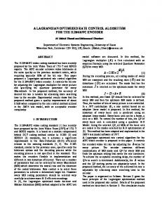
Figure 1: Transmission configuration of FREWL.
are introduced to solve the objective function. In Section 4, the effectiveness of OTCM is verified by simulation analysis. In Section 5, we discussed the applicability of OTCM and analyzed the reason for different simulation results of four algorithms.
2. Dynamical Model of FREWL The distinctive transmission configuration of FREWL takes diesel generating set as main power source. Rectifier converts the alternating current generated by diesel generating set to a direct current which used to drive front motor, rear motor, and working motor. Supercapacitor is used as auxiliary source to effectively use braking energy and control diesel generating set in its high efficiency operating region. So diesel generating set can always operate in its high efficiency region. The transmission configuration of FREWL is shown in Figure 1. A brief summary of the forces and torques in longitudinal dynamics is shown in Figure 2. 2.1. Wheel Vertical Load. Because FREWL operates in low speed, the influence of air resistance can be ignored. The wheel vertical load is, respectively, given by 𝐹𝑧𝑓 = 𝐹𝑧𝑟 =
𝑚V̇𝑥 ℎ − 𝑚𝑔ℎ sin 𝛼 + 𝑚𝑔𝑙𝑟 cos 𝛼 + 𝐹𝑧 𝑙𝑧 𝑙𝑓 + 𝑙𝑟 −𝑚V̇𝑥 ℎ + 𝑚𝑔ℎ sin 𝛼 + 𝑚𝑔𝑙𝑓 cos 𝛼 − 𝐹𝑧 𝑙𝑐 𝑙𝑓 + 𝑙𝑟
where 𝑙𝑓 is the distance from FREWL gravity center to front axle, 𝑙𝑟 is the distance from FREWL gravity center to rear axle, 𝑙𝑐 is the distance from the front axle to the tooth tip of bucket, 𝑙𝑧 = 𝑙𝑐 + 𝑙𝑓 + 𝑙𝑟 , ℎ is the height of FREWL gravity center, 𝑚 is the mass, 𝛼 is the gradient of the slope, V̇𝑥 is the longitudinal acceleration, 𝐹𝑧𝑓 and 𝐹𝑧𝑟 are the vertical loads of front and rear wheels, 𝐹𝑧 is the vertical component of spading resistance on the tooth tip of bucket, and 𝐹𝑥 is the horizontal component of spading resistance on the tooth tip of bucket. 2.2. Tire Driving Torque and Wheel Longitudinal Force. The relationship between the longitudinal force and driving torque on each tire is given by 𝐼𝑒 𝜔̇ 𝑤𝑖 = 𝑇𝑖 − 𝑟eff 𝐹𝑥𝑖 ,
where 𝐼𝑒 is the wheel rotational inertia, 𝑟eff is the tire rolling radius, 𝜔̇ 𝑤𝑖 is the wheel angular acceleration, 𝐹𝑥𝑖 is the wheel longitudinal force, and 𝑇𝑖 is the tire driving torque. 𝑖 in subscript denotes the front or rear axle. 2.3. Motor Driving Torque. Suppose that longitudinal force and vertical load of the wheels in the same axle are equal; the relationship between the motor driving torque and tire driving torque is given by 2𝑇𝑖 (3) + 𝐼𝑚 𝜔̇ 𝑚𝑖 , 𝑁 where 𝑇𝑚𝑖 is the motor driving torque, 𝐼𝑚 is the motor rotational inertia, 𝜔̇ 𝑚𝑖 is the motor angular acceleration, and 𝑁 is the reduction ratio from the motor to the wheels. 𝑇𝑚𝑖 =
(1) ,
(2)
Mathematical Problems in Engineering
3
x ẋ Tf
Tr
mg sin ℎ
Fx
Fxf
Fz
lc
Fzf
lf l mg cos
lr
Fxr Fzr
Figure 2: Illustration of FREWL forces and torques.
𝑇𝑚𝑟 is the driving torque of the rear motor. Tire workload of each wheel is defined as
3. Optimal Torque-Distribution Control Method
𝜅2 𝑇𝑚2 𝑁2
OTCM consists of objective function, constraint conditions, and optimization algorithm.
𝛾𝑓𝑙 = 𝛾𝑓𝑟 =
3.1. Objective Function
(1 − 𝜅)2 𝑇𝑚2 𝑁2 𝛾𝑟𝑙 = 𝛾𝑟𝑟 = , 4𝑟eff 2 𝜇𝑟 2 𝐹𝑧𝑟 2
3.1.1. Optimized Torque-Distribution Control Based on Tire Workload. The nonlinear optimization problem about enhancing operating performance can be formulated in this way. Because of the characteristic that the driving torque of both motors can be controlled online, the objective function is that the weighted sum of variance and mean of tire workload is minimal [5]. It can be defined as min 𝐽 = var (𝛾𝑖 ) + 𝜀V 𝐸 (𝛾𝑖 ) 1 4 2 = ∑ (𝛾𝑖 − 𝐸 (𝛾𝑖 )) + 𝜀V 𝐸 (𝛾𝑖 ) . 4 𝑖=1 as
(4)
From (2) and (3), tire workload 𝛾𝑖 of each wheel is defined 𝛾𝑖 =
2 𝑁2 𝑇𝑚𝑖
4𝑟eff 2 𝜇𝑖 2 𝐹𝑧𝑖 2
,
(5)
where 𝜇𝑖 is the tire-road friction coefficient of each wheel and 𝑁 is the reduction ratio. By the characteristic that the driving torque of both front motor and rear motor can be controlled online, the objective function can be set by the minimum of weighted sum of variance and mean of tire workload. Distribution coefficient 𝜅 is defined as 𝜅=
𝑇𝑚𝑓 𝑇𝑚𝑓 + 𝑇𝑚𝑟
=
𝑇𝑚𝑓 𝑇𝑚
,
(6)
where 𝑇𝑚 is the sum of driving torque of the front motor and rear motor, 𝑇𝑚𝑓 is the driving torque of the front motor, and
4𝑟eff 2 𝜇𝑓 2 𝐹𝑧𝑓 2
(7)
where 𝛾𝑓𝑙 is the tire workload of left-front wheel, 𝛾𝑓𝑟 is the tire workload of the right-front wheel, 𝛾𝑟𝑙 is the tire workload of left-rear wheel, and 𝛾𝑟𝑟 is the tire workload of right-rear wheel. 3.1.2. Optimized Torque-Distribution Control Based on Total Motor Efficiency. In order to improve the energy efficiency of the FREWL while transferring equipment, the objective function is that the total motor efficiency is maximal [12]. It can be defined as 𝑇𝑚 𝑛 , (8) max 𝜂 = 2 [𝑇𝑚𝑓 /𝜂𝑓 (𝑇𝑚𝑓 , 𝑛𝑓 ) + 𝑇𝑚𝑟 /𝜂𝑟 (𝑇𝑚𝑟 , 𝑛𝑟 )] 𝑛 where 𝜂𝑓 is the efficiency of front motor, 𝜂𝑟 is the efficiency of rear motor, 𝑛𝑓 is the front motor speed, and 𝑛𝑟 is the rear motor speed. The relationship between motor efficiency 𝜂𝑓 , motor torque 𝑇𝑓 , and motor speed 𝑛𝑓 is shown in Figure 3. With (6), then (8) becomes max
𝜂=
1 𝜅/𝜂𝑓 (𝑇𝑚𝑓 , 𝑛𝑓 ) + (1 − 𝜅) /𝜂𝑟 (𝑇𝑚𝑟 , 𝑛𝑟 )
.
(9)
3.2. Constraint Conditions. The total driving torque should satisfy expected accelerator position firstly, as is shown in 𝑇𝑚 = 𝑓 (𝜕pedal , 𝑛) ,
(10)
where 𝜕pedal is the accelerator position and 𝑛 is the motor speed. The surface about the three parameters is shown as Figure 4.
4
Mathematical Problems in Engineering 90 80
80 60 40 20 0
1000
180 160 140 120 100 80 60 40 20
Torq ue ( Nm )
Efficiency (%)
70
3000
5000 Rotate s peed (r
7000 pm)
60 50 40 30 20
𝑇 𝑓 (𝑥) ≈ 𝑓 (𝑥𝑘+1 ) + 𝑔𝑘+1 (𝑥 − 𝑥𝑘+1 )
1 𝑇 (𝑥 − 𝑥𝑘+1 ) 𝐺𝑘+1 (𝑥 − 𝑥𝑘+1 ) . 2 The derivative of (14) is +
90 Total output torque of front and rear motor (Nm)
3.3.1. Quasi-Newton Lagrangian Multiplier Method. QuasiNewton method (QNM) is a special case of Newton method. The objective function is Taylor expanded in second order at 𝑥𝑘+1 , as shown in (14).
9000
Figure 3: MAP diagram of motor.
90 80 70 60 50 40 30 20 10 0 100 80 60 40 Throt 20 0 tle pe da l de gree ( %)
sequential quadratic programming (SQP), adaptive genetic algorithms (AGA), and particle swarm optimization with random weighting and natural selection, (PSO-RN). The notable advantage that these four algorithms possess over their classic one is the fast solution speed, which satisfies the requirement of subsequent field test of FREWL.
𝑔 (𝑥) ≈ 𝑔𝑘+1 + 𝐺𝑘+1 (𝑥 − 𝑥𝑘+1 ) .
80 70 60 50
𝐵𝑘+1 = 𝐵𝑘 −
30 20 0
10 0
Figure 4: Defining surface of total driving torque of front/rear motor.
(15)
An approximate matrix 𝐵𝑘 is used to replace 𝐺𝑘+1 in (15). The Broyden-Fletcher-Goldfarb-Shanno (BFGS) is used to update the 𝐵𝑘 , as shown in (16).
40
2500 1500 2000 500 1000 ) m p eed (r Motor sp
(14)
𝐵𝑘 𝑠𝑘 𝑠𝑘𝑇 𝐵𝑘 𝑦𝑘 𝑦𝑘𝑇 + 𝑇 . 𝑠𝑘𝑇 𝐵𝑘 𝑠𝑘 𝑦𝑘 𝑠𝑘
(16)
Quasi-Newton method fails to solve the nonlinear constraints optimization problems. Thus Lagrangian multiplier (LM) is introduced into the problem. Inequality constraints are transformed into equality constraints by an auxiliary variable. Then with the original equality constraints, the Lagrangian function is transformed into 𝜓 (𝑥, 𝑦, 𝜆, 𝜎)
Adhesion force is influenced by wheel vertical load and tire-road friction coefficient. Because the influence of the motor inertia moment and wheel inertia moment is tiny, it is appropriate to ignore them. So in pure longitudinal slip condition, the maximum driving torque is limited by 2𝜇𝑖,𝑥 𝐹𝑖,𝑧 𝑟eff . 𝑇𝑚𝑖 ≤ 𝑁
(11)
The motor driving torque and speed should be limited as follows: 𝑇𝑚𝑖 ≤ 𝑇max (12) 𝑛 ≤ 𝑛max . The range of driving torque-distribution coefficient 𝜅 is given by 0 ≤ 𝜅 ≤ 1.
(13)
3.3. Optimization Algorithms. Nonlinear optimization algorithms are widely used to solve nonlinear optimization problems [28]. Each nonlinear optimization algorithm has its capabilities and limitations, which have a significant impact on the performance of OTCM. The common optimization algorithms for nonlinear constraints optimization problems are quasi-Newton Lagrangian multiplier method (QNLM),
where the iterative equation of the multiplier is (𝜇𝑘+1 )𝑖 = (𝜇𝑘 )𝑖 − 𝜎ℎ𝑖 (𝑥𝑘 ) , 𝑖 = 1, 2, . . . , 𝑙, (𝜆 𝑘+1 )𝑖 = max {0, (𝜆 𝑘 )𝑖 − 𝜎𝑔𝑖 (𝑥𝑘 )} , 𝑖 = 1, 2, . . . , 𝑚.
(18)
The termination criterion of iteration is 𝑙
(∑ℎ𝑖2 𝑖=1
𝑚
2
1/2
(𝜆 𝑘 )𝑖 (𝑥𝑘 ) + ∑ [min {𝑔𝑖 (𝑥𝑘 ) , }] ) 𝜎 𝑖=1
≤ 𝜀, (19)
where 𝜆 is called a multiplier, 𝜎 is penalty factor, and 𝜀 is termination error ranging from 0 to 1. The simulation parameters of the QNLM used in this paper are shown in Table 2. QNLM consists of QNM and LM. QNM and LM have their own maximum iteration number and termination error. The maximum iteration and termination error have influence on the computing accuracy and computing time. Penalty factor 𝜎 is used to penalize those individuals which do not satisfy the constraint condition for solving constrained optimization problems.
Mathematical Problems in Engineering
5
Table 2: Simulation parameters of the QNLM. Parameters Maximum iteration number of QNM Maximum iteration number of LM Penalty factor of LM Termination error of QNM Termination error of LM
3.3.2. Sequential Quadratic Programming. SQP is an efficient method for nonlinear optimization with advantages of high computational efficiency and fast convergent rate. In SQP, positive definite matrix 𝐵0 ∈ 𝑅𝑛×𝑛 is used to seek the optimal solution 𝑑𝑘 of subquestion. The subquestion is described as min s.t.
𝑇
ℎ (𝑥𝑘 ) + ∇ℎ (𝑥𝑘 ) 𝑑 = 0,
(20)
𝑇
𝑔 (𝑥𝑘 ) + ∇𝑔 (𝑥𝑘 ) 𝑑 ≥ 0. If the constraints ‖𝑑𝑘 ‖1 ≤ 𝜀1 and ‖ℎ𝑘 ‖1 + ‖(𝑔𝑘 )− ‖1 ≤ 𝜀2 are satisfied, the calculation will be determined. [𝑔𝑘 (𝑥)]− = max{0, −𝑔𝑘 (𝑥)}, and 1 means the initial value. A point under Karush–Kuhn–Tucker (KKT) condition is obtained and the termination error is 0 ≤ 𝜀1 , 𝜀2 ≤ 1. To some value function 𝜙(𝑥, 𝜎), the chosen penalty factor 𝜎 defines that 𝑑𝑘 is decreasing at the point 𝑥𝑘 . Suppose that 𝑚 𝑘 is the tiniest nonnegative integer satisfying the following equation: 𝜙 (𝑥𝑘 + 𝜌𝑚 𝑑𝑘 , 𝜎𝑘 ) − 𝜙 (𝑥𝑘 , 𝜎𝑘 ) ≤ 𝜂𝜌𝑚 𝜙 (𝑥𝑘 , 𝜎𝑘 ; 𝑑𝑘 ) ,
(21)
where 𝜂 ∈ (0, 1/2) and 𝜌 ∈ (0, 1). From 𝛼𝑘 = 𝜌𝑚𝑘 , 𝑥𝑘+1 = 𝑥𝑘 + 𝛼𝑘 𝑑𝑘 , 𝐴 𝑘+1 is given by 𝑇 𝑇
𝐴 𝑘+1 = (∇ℎ (𝑥𝑘+1 ) , ∇𝑔 (𝑥𝑘+1 ) ) .
(22)
The least square multiplier is calculated by (
𝜇𝑘+1 𝜆 𝑘+1
)=
−1 [𝐴 𝑘+1 𝐴𝑇𝑘+1 ]
Values
Maximum iteration number
200
Iteration number of subproblem
200
Penalty factor Termination error
0.05 1𝑒 − 5
Termination error of subproblem
1𝑒 − 5
Table 4: Simulation parameters of the AGA. Parameters
Values
Lower bound of independent variable
1
Upper bound of independent variable
0
Scale of population
1 𝑇 𝑇 𝑑 𝐵𝑘 𝑑 + ∇𝑓 (𝑥𝑘 ) 𝑑, 2
𝑇
Parameters
𝐴 𝑘+1 ∇𝑓 (𝑥𝑘+1 ) .
(23)
The approximate matrix 𝐵𝑘 is the same as in (16). The simulation parameters of the SQP used in this paper are shown in Table 3. SQP needs to solve a quadratic programming subproblem at every iteration step. It is necessary to set its and subproblem’s maximum iteration number and termination error. The values of maximum iteration number, termination error, and penalty factor are the same as the function in QNLM. 3.3.3. Adaptive Genetic Algorithms. AGA is another significant and promising variant of genetic algorithms. AGA adjusts probabilities of crossover and probabilities of mutation in order to maintain the genetic model and to accelerate the convergence speed. In AGA, the evolution usually starts
Maximum evolution generations Discrete precision of independent variable Crossover constant 𝑘1 Crossover constant 𝑘2 Mutation constant 𝑘3 Mutation constant 𝑘4
50 200 1𝑒 − 5 0.5 0.9 0.03 0.07
from a population which consisted of randomly generated individuals. By Roulette strategy, individual fitness values are evaluated to judge if it agrees with the optimization criterion. The new individuals are generated by the optimal best mutation probability 𝑃𝑚 and the best crossover probability 𝑃𝑐 whose equations are shown in 𝑘 (𝑓 − 𝑓) { { 1 max , 𝑓 ≥ 𝑓avg 𝑃𝑐 = { 𝑓max − 𝑓avg { 𝑓 < 𝑓avg {𝑘2 , 𝑘 (𝑓 − 𝑓 ) { { 3 max , 𝑓 ≥ 𝑓avg 𝑃𝑚 = { 𝑓max − 𝑓avg { 𝑓 < 𝑓avg , {𝑘4 ,
(24)
where 𝑓max is the maximum fitness value population, 𝑓avg is the mean fitness value population, 𝑓 is the bigger fitness value in two individuals about to crossover, and 𝑓 is the fitness value of individuals about to mutate. 𝑘1 , 𝑘2 , 𝑘3 , and 𝑘4 are the constants. The simulation parameters of AGA used in this paper are shown in Table 4. Among them, the lower bound and upper bound of independent variable and discrete precision determine the encoding length required for the binary encoding. The values for lower bound and upper bound depend on the constraints. The scale of population and the maximum ecology affect the accuracy and computing time. In order to analyze the advantages and disadvantages of the various algorithms as much as possible, the maximum evolution generations are the same with the maximum number of the same number of QNLM and SQP. The values of 𝑘1 , 𝑘2 , 𝑘3 , and 𝑘4 are usually based on different application objects. It generally requires that 𝑘1 < 𝑘2 , 𝑘3 < 𝑘4 .
6
Mathematical Problems in Engineering Table 5: Simulation parameters of the PSO-RN. Values
Particle population Acceleration constant 𝑐1
30 2
Acceleration constant 𝑐2 Upper boundary of inertia weight Lower boundary of inertia weight
0.9 0.4
Maximum evolution generations Dimension of search space
2
Maximum particle velocity Vmax Minimum particle velocity Vmin Maximum particle position 𝑥max
100 1 0.2 0 1
Minimum particle position 𝑥min
0
3.3.4. Particle Swarm Optimization with Random Weighting and Natural Selection. Particle swarm optimization (PSO) based on natural selection is one of the improved algorithms, which is characterized by iteratively trying to improve a candidate solution. In each iteration, the worst half of the particles in the population is replaced by the best half of the particles while preserving the original historical optimal value. Therefore, it improves the optimization ability and solving speed and significantly reduces the algorithm premature convergence situation. The inertia weight 𝛼 is an important parameter in the PSO which is used to control the ability of development and search. The core of avoiding falling into the local optimal is to determine a reasonable inertia weight. In order to accelerate up the convergence speed, the inertia weight 𝛼 is set as a random value. The equation to calculate the random 𝛼 is 𝜔 = 𝛼 + 𝜎 × 𝑁 (0, 1) 𝛼 = 𝛼min + (𝛼max − 𝛼min ) × rand (0, 1) ,
(25)
where 𝜎 is the random weight, 𝛼max and 𝛼min are the maximum and minimum of the inertia weight, and 𝑁(0, 1) is the random number of standard state distribution. The simulation parameters of the PSO-RN used in this paper are shown in Table 5. Acceleration constants 𝑐1 and 𝑐2 determine the influence of particle individual experience and group experience on the trajectory of particle movement, usually 𝑐1 = 𝑐2 . Inertia weight can be used to control the algorithm development and search capabilities, which have different values according to different application problems. Dimension of search space has the same value as the number of its independent variables. Maximum particle position 𝑥max and minimum particle position 𝑥min are the boundary conditions of the algorithm, and the numerical value depends on the constraints of the actual problem. Maximum particle velocity Vmax determines the maximum distance that the particle can move in one flight, usually Vmax = 𝑘𝑥max , 0.1 ≤ 𝑘 ≤ 1.
𝜇𝑓 𝜇𝑟 𝑇𝑚 (Nm) 𝐹𝑥 (N) 𝛼 (∘ ) 1
Condition 1 0.8 0.3 300 — —
Condition 2 0.2 0.7 300 600 —
Condition 3 0.2 0.2 360 600 20
0.3243 0.3243 0.3243
0.8 Longitudinal slip ratio
Parameters
Table 6: Simulation parameters based on tire workload.
0.3243 0.3243 0.3243
0.6
0.3243 0.3243 0.3243
0.4
6.956
6.957
6.958
6.959
6.96
0.2
0
0
5
QNLM SQP AGA
10 Time (s)
15
20
PSO-RN No-control
Figure 5: Longitudinal slip ratio of front wheel.
4. Simulation Results 4.1. Simulation of OTCM Based on Tire Workload. Conditions of traveling, spading, and stacking on bumpy road are common for wheel loader. The paper establishes these three conditions to verify the improvement of the FREWL operation performance through OTCM based on tire workload. Condition 1 simulates the traveling condition, while condition 2 simulates the spading condition. Condition 3 simulates the stacking condition in bumpy road with 20∘ slope. The simulation parameters are listed in Table 6. From Figures 5 and 6, it is notable that in the first 2 s, namely, the starting stage, the longitudinal slip ratio of controlled FREWL is much smaller than no-control FREWL. The operation performance has significantly improved by OTCM. After 3 s, namely, the driving stage, the longitudinal ratio optimized by AGA is smoother than other three algorithms, so the operation performance of FREWL is the best. Another parameter to evaluate the control effect is the driving distance of the controlled FREWL and no-control FREWL on bumpy road in the same time, which is shown in Figure 7. Table 7 shows the driving distance of the FREWL without spading. Controlled FREWL has better control to longitudinal slip ratio; thus it marches earlier and drives farther than no-control FREWL. The OTCM based on AGA has the best control effect, and the driving distance compared
7
1
1
0.8
0.8 Longitudinal slip ratio
Longitudinal slip ratio
Mathematical Problems in Engineering
0.6
0.4
0.2
0
0.6
0.4
0.2
0
5
10 Time (s)
QNLM SQP AGA
15
0
20
0
5
10 Time (s)
QNLM SQP AGA
PSO-RN No-control
Figure 6: Longitudinal slip ratio of rear wheel.
15
20
PSO-RN No-control
Figure 8: Longitudinal slip ratio of front wheel.
25
1
13.865
20 0.8
15
Longitudinal slip ratio
Driving distance (m)
13.86
13.855
10
13.85
15.964
15.966
15.968
15.97
5 0 −5
0.6
0.4
0.2
0
5
10 Time (s)
QNLM SQP AGA
15
20
PSO-RN No-control
Figure 7: Driving distance in condition 1.
0
0
5
QNLM SQP AGA
10 Time (s)
15
20
PSO-RN No-control
Figure 9: Longitudinal slip ratio of rear wheel.
Table 7: Driving distance without spading resistance. No-control SQP AGA PSO-RN QNLM
Final distance (m) 16.92 19.53 20.08 19.54 19.54
Distance increase (%) — 15.42 18.68 15.48 15.48
to no-control FREWL is increased by 18.68%. The control effect of other three optimization algorithms is basically the
same; the driving distance is increased by 15.48% compared to the no-control FREWL. Figures 8 and 9 show the longitudinal slip ratio of front and rear wheel in condition 2, respectively. Table 8 shows slip frequency of the front and rear wheel of the controlled FREWL and no-control FREWL. In whole simulation time, especially the starting stage, the control effect of OTCM based on SQP is the best. Only the rear wheel slips once. Figure 10 shows the driving distance of FREWL in condition 2. Controlled FREWL utilizes adhesion ability better
8
Mathematical Problems in Engineering 1
Table 8: Slip frequency of the front and rear wheels. Rear wheel slip times 1 1 4 1 1
Table 9: Forward driving time with spading resistance.
No-control SQP AGA PSO-RN QNLM
Driving time (s) 15.42 3.98 8.42 3.92 3.96
0.8 Longitudinal slip ratio
No-control SQP AGA PSO-RN QNLM
Front wheel slip times 4 0 2 0 0
Time decrease (%) — 74.19 45.39 74.59 74.32
0.6
0.4
0.2
0
0
0.5
15
20
PSO-RN No-control
Figure 11: Longitudinal slip ratio of front wheel.
and slips less and also can go forward in a shorter period when encountering spading resistance, as shown in Table 9. In this case, FREWL controlled by QNLN, SQP, and PSORN can go forward in a shorter period and make significant improvement, but the control effect of OTCM based on AGA is undesirable. Condition 3 simulates stacking condition that the FREWL operates on the bumpy road with 20∘ slope and encounters a continuous spading resistance after 5 s, and is gradually heavy-loaded. Compared to conditions 1 and 2, condition 3 is more complicated. Figures 11 and 12 show the longitudinal slip ratio of front and rear wheel in condition 3. It is obvious that after 10 s the front wheel of no-control FREWL is basically in the slippery state. While the FREWL applies four optimization algorithms, the slippery time is much less.
QNLM SQP AGA
10 Time (s)
15
20
PSO-RN No-control
Figure 12: Longitudinal slip ratio of rear wheel.
Among them, AGA-controlled FREWL slips the least. The control effects of the other three algorithms are similar. Figure 13 shows the driving distance of FREWL in condition 3. Since AGA is better in control of the longitudinal slip ratio of front/rear wheel in Figures 11 and 12, it drives farthest. The other three algorithms also have a good performance compared to no-control. This shows that FREWL, which applied OTCM based on tire workload, has better operation performance in stacking condition than no-control FREWL.
9
6
70
5
60
4
50 Efficiency (%)
Driving distance (m)
Mathematical Problems in Engineering
3 4.55
2
4.5
−1
4.35
0
49.396 49.394 49.392
4.4
0
49.4 49.398
30
4.45
1
40
49.39
20
49.388
10 10.1 10.2 10.3 10.4 10.5 10.6
5
10 Time (s)
QNLM SQP AGA
8.47 8.472 8.474 8.476 8.478 8.48
15
10
20
0
5
10
15
Time (s) QNLM SQP AGA
PSO-RN No-control
Figure 13: Driving distance in condition 3.
PSO-RN No-control
Figure 14: Total motor efficiency in condition 4. 15
Table 10: Simulation parameters based on total motor efficiency. Condition 4 Straight driving 0.8 0.8 0 100
Condition 5 Reciprocating driving 0.6 0.6 10 200
Table 11: Total motor efficiency in straight driving.
No-control SQP AGA PSO-RN
Maximum total motor efficiency (%)
Efficiency increase (%)
43.63 49.58 49.57 50.12
— 13.64 13.48 14.86
4.2. Optimized Torque-Distribution Control Based on Total Motor Efficiency. Two most common equipment transferring conditions are driving straightly on the bituminous road and reciprocating on bumpy road. This paper sets two conditions to simulate the improvement of energy efficiency of FREWL by OTCM while transferring equipment. The simulation parameters are listed in Table 10. Condition 4 is set to observe the energy efficiency of FREWL while driving straightly on the bituminous road. Condition 5 is set to observe the energy efficiency of FREWL while reciprocating on bumpy road. Figure 14 shows the total motor efficiency of the FREWL when the FREWL is traveling on the bituminous road. Table 11 shows the maximum motor efficiency of the various optimization algorithms. The total motor efficiency optimized by OTCM based on QNLM fluctuates frequently
10 Longitudinal speed (km/h)
Motion state 𝜇𝑓 𝜇𝑟 V0 (m/s) 𝑇𝑚 (Nm)
9.7 9.6 9.5 9.4 9.3 9.2 9.1 9
5
0
−5
−10
7.35
0
7.4
7.45
5
7.5
10
15
Time (s) SQP AGA
PSO-RN No-control
Figure 15: Longitudinal speed in condition 5.
and violently in the starting stage of simulation, which leads to calculation failure, which means that QNLM is not suitable for problems with strong-nonlinearity. The results of other three optimization algorithms are better than no-control FREWL. The PSO-RN works best; the total motor efficiency is increased by 14.86% comparing to no-control FREWL. The results of SPQ and AGA are roughly the same; the total motor efficiency is increased by 13.64% comparing to no-control FREWL. Figures 15 and 16 show longitudinal speed and total motor efficiency of FREWL in condition 5. Table 12 shows the maximum total motor efficiency of FREWL in the forward
10
Mathematical Problems in Engineering Table 12: Total motor efficiency in reciprocating driving.
No-control SQP AGA PSO-RN
Forward-total motor efficiency (%)
Forward-efficiency increase (%)
Backward-total motor efficiency (%)
Backward-efficiency increase (%)
46.53 53.62 51.68 52.25
— 15.24 11.07 12.29
28.61 36.02 36.94 34.52
— 25.90 29.12 20.66
70
Table 13: Simulation time of OTCM on different conditions.
QNLM (s) SQP (s) AGA (min) PSO-RN (min) 32.7 55.6 69.2 27.3 23.5 36.1 88.3 54.8 32.1 41.6 64.9 29.5 — 17.9 52.7 15.7 — 13.9 54.7 18.1
0
5
10
15
Time (s) SQP AGA
PSO-RN No-control
Figure 16: Total motor efficiency in condition 5.
stage and the backward stage. The total motor efficiency of controlled FREWL is greatly improved compared to nocontrol FREWL when driving reciprocally. The results by OTCM perform better in backward stage than in forward stage. The solution of SQP is the best in forward stage; the total motor efficiency is increased by 15.24% at most. The result of AGA works best in backward stage; the total motor efficiency is increased by 29.12% at most. 4.3. Simulation Time. Simulation time is an essential factor to affect the practicability of the method. Table 13 shows the simulation time of the optimization algorithms under various conditions. The simulation step size is 0.001 s in the Simulink/Carsim platforms. Taking into account the actual real test, the sampling step is generally set to 0.01 s. Therefore, QNLM and SQP can be used in the online control, but AGA and PSO-RN cannot. Because QNLM fails in equipment transferring condition, SQP is comprehensively the best optimization algorithm for OTCM in actual test.
5. Discussion In this paper, we study the OTCM of FREWL and prove that OTCM can improve the operation performance and energy efficiency of FREWL through five simulation conditions. In addition to five simulation conditions mentioned in this
Heavy-haul transportation Loading/unloading material Bulldozing Climbing
𝑚 ✓ ✓ ✓ —
𝛼 — — — ✓
V̇𝑥 ✓ ✓ ✓ ✓
𝐹𝑥 — ✓ ✓ —
𝐹𝑧 — ✓ ✓ —
paper, this method is also adaptable to other operation and equipment transferring conditions of FREWL in longitudinal motion. The changed parameters are shown in Table 14. Tick “✓” means this parameter is changed in that situation and hyphen “—” means it is unchanged. As can be seen from Table 14, in other conditions, all the changed parameters are taken into account in the dynamic model of FREWL. At the same time, the optimization algorithm and optimization goals do not change. Therefore, the method proposed in this paper is suitable for operation and equipment transferring conditions. In the simulation case, compared to no-control FREWL, the FREWL controlled by four optimization algorithms have a great increase in the operation performance and energy efficiency. In the OTCM based on tire workload, the QNLM and SQP optimization solutions are almost identical, because their core algorithm is the BFGS algorithm, as shown in (16). PSO-RN and AGA are modern intelligent optimization algorithms, but their results are quite different because the optimal solution of PSO-RN is easy to fall into the local optimal solution. Comparing to PSO-RN, AGA increases the crossover probability and mutation probability when the optimal solution tends to local optimal solution, enhancing the ability to solve the global optimal solution. Thus, AGA generally has a better performance in most simulation conditions. However, although the AGA has a better performance, it has the longest computing time because the movement of the whole population is more evenly moving to the optimal region. QNLM and SQP compute faster because they apply
Mathematical Problems in Engineering
11
the traditional BFGS method. Among them, SQP needs to solve a quadratic programming subproblem at each iteration step, so the calculation time is longer than QNLM. [7]
6. Conclusion OTCM is a critical technology to improve the operation performance and energy efficiency of FREWL. The driving torque of front motor and rear motor of FREWL can be controlled independently. The objective function minimizes the weighted sum of variance and mean value of tire workload and maximizes the total motor efficiency. The results show that the operation performance and energy efficiency are obviously improved by OTCM. While the FREWL is operating, the frequency of slip is obviously reduced, and the adhesion ability is improved. While the FREWL is driving straightly in equipment transferring, total motor efficiency is improved by 14.86% at most. While the FREWL is driving reciprocally in equipment transferring, total motor efficiency is improved by 29.12% at most. Considering the simulation results and simulation time comprehensively, SQP is the most suitable one of the four optimization algorithms for field test of FREWL.
[8]
[9]
[10]
[11]
[12]
Conflicts of Interest The authors declare that there are no conflicts of interest regarding the publication of this paper.
[13]
Acknowledgments The authors acknowledge the funding support from National Natural Science Foundation of China, no. 51375202, and also acknowledge the support of Programs for Science Research and Development of Jilin Province, no. 20160101285JC.
[14]
[15]
References [1] Z. Naiwei, D. Qunliang, J. Yuanhua, Z. Wei, and R. Youcun, “Modeling and simulation research of coaxial parallel hybrid loader,” Applied Mechanics and Materials, vol. 29–32, pp. 1634– 1639, 2010. [2] J. Wang, Z. Yang, S. Liu, Q. Zhang, and Y. Han, “A comprehensive overview of hybrid construction machinery,” Advances in Mechanical Engineering, vol. 8, no. 3, pp. 1–15, 2016. [3] F. Wang, M. A. Mohd Zulkefli, Z. Sun, and K. A. Stelson, “Energy management strategy for a power-split hydraulic hybrid wheel loader,” Proceedings of the Institution of Mechanical Engineers, Part D: Journal of Automobile Engineering, vol. 230, no. 8, pp. 1105–1120, 2016. [4] P. Song, M. Tomizuka, and C. Zong, “A novel integrated chassis controller for full drive-by-wire vehicles,” Vehicle System Dynamics, vol. 53, no. 2, pp. 215–236, 2015. [5] Y. Dai, Y. Luo, W. Chu, and K. Li, “Optimum tyre force distribution for four-wheel-independent drive electric vehicle with active front steering,” International Journal of Vehicle Design, vol. 65, no. 4, pp. 336–359, 2014. [6] H. Fujimoto and K. Maeda, “Optimal yaw-rate control for electric vehicles with active front-rear steering and four-wheel driving-braking force distribution,” in Proceedings of the 39th
[16]
[17]
[18]
[19]
[20]
Annual Conference of the IEEE Industrial Electronics Society (IECON ’13), pp. 6514–6519, IEEE, Vienna, AUSTRIA, November 2013. J. Kim, “Optimal power distribution of front and rear motors for minimizing energy consumption of 4-wheel-drive electric vehicles,” International Journal of Automotive Technology, vol. 17, no. 2, pp. 319–326, 2016. A. Pennycott, L. De Novellis, A. Sabbatini, P. Gruber, and A. Sorniotti, “Reducing the motor power losses of a fourwheel drive, fully electric vehicle via wheel torque allocation,” Proceedings of the Institution of Mechanical Engineers, Part D: Journal of Automobile Engineering, vol. 228, no. 7, pp. 830–839, 2014. T. Cheong, S. H. Song, and C. Hu, “Strategic alliance with competitors in the electric vehicle market: tesla motor’s case,” Mathematical Problems in Engineering, vol. 2016, Article ID 7210767, 10 pages, 2016. H. He, J. Fan, Y. Li, and J. Li, “When to switch to a hybrid electric vehicle: a replacement optimisation decision,” Journal of Cleaner Production, vol. 148, pp. 295–303, 2017. Y. Suzuki, Y. Kano, and M. Abe, “A study on tyre force distribution controls for full drive-by-wire electric vehicle,” Vehicle System Dynamics, vol. 52, no. 1, pp. 235–250, 2014. Z.-P. Yu, L.-J. Zhang, and L. Xiong, “Optimized torque distribution control to achieve higher fuel economy of 4WD electric vehicle with four in-wheel motors,” Journal of Tongji University, vol. 33, no. 10, pp. 79–85, 2005. D. Wang and B. Wang, “Research on driving force optimal distribution and fuzzy decision control system for a dual-motor electric vehicle,” in Proceedings of the 34th Chinese Control Conference (CCC ’15), pp. 8146–8153, IEEE, Hangzhou, China, July 2015. A. F. Izmailov, M. V. Solodov, and E. I. Uskov, “Globalizing stabilized sequential quadratic programming method by smooth primal-dual exact penalty function,” Journal of Optimization Theory and Applications, vol. 169, no. 1, pp. 148–178, 2016. M. A. Z. Raja, A. Zameer, A. U. Khan, and A. M. Wazwaz, “A new numerical approach to solve Thomas–Fermi model of an atom using bio-inspired heuristics integrated with sequential quadratic programming,” SpringerPlus, vol. 5, no. 1, article 1400, 2016. J. Apolinar and M. Rodr´ıguez, “Three-dimensional microscope vision system based on micro laser line scanning and adaptive genetic algorithms,” Optics Communications, vol. 385, pp. 1–8, 2017. B. Bao, Y. Yang, Q. Chen, A. Liu, and J. Zhao, “Task allocation optimization in collaborative customized product development based on double-population adaptive genetic algorithm,” Journal of Intelligent Manufacturing, vol. 27, no. 5, pp. 1097–1110, 2016. Y. Chen and M. S. Li, “A harmonic parameter estimation method based on Particle Swarm Optimizer with Natural Selection,” in Proceedings of the 1st International Conference on Information and Communication Technology Research (ICTRC ’15), pp. 206–209, IEEE, Abu Dhabi, Arab Emipates, May 2015. Y. Hu, J. Lu, Y. Deng, and Z. Zhang, “MPPT algorithm based on particle swarm optimization with natural selection,” in Proceedings of the 3rd International Conference on Machinery, Materials and Information Technology Applications (ICMMITA ’15), pp. 1814–1817, Atlantis Press, Qingdao, China, November 2015. H. Inoue, “Introduction of PC200-8 hybrid hydraulic excavators,” Report, Komatsu, vol. 54, no. 161, pp. 1–6, 2008.
12 [21] M. Ochiai and S. Ryu, “Hybrid in construction machinery,” in Proceedings of the 7th JFPS international symposium on fluid power, pp. 41–44, Toyama, Japan, September 2008. [22] M. Ochiai, “Technical trend and problem in construction machinery,” Construction Machinery, vol. 38, no. 4, pp. 20–24, 2002. [23] S. Riyuu, M. Tamura, and M. Ochiai, “Hybrid construction machine,” Patent 2003328397, Japan, 2003. [24] J. Deere, “644K Hybrid Wheel Loader,” 2017, http://www.deere .com/wps/dcom/en US/products/equipment/wheel loaders/ 644k hybrid/644k hybrid.page. [25] J. Global, “L-950 Wheel Loader,” 2017, https://mining.komatsu/ product-details/l-950#!technology. [26] S. Hui and J. Junqing, “Research on the system configuration and energy control strategy for parallel hydraulic hybrid loader,” Automation in Construction, vol. 19, no. 2, pp. 213–220, 2010. [27] N. Zhou, E. Zhang, Q. Wang et al., “Compound hybrid wheel loader,” Patent CN102653228A, China, 2012. [28] M. P. Aghababa, “3D path planning for underwater vehicles using five evolutionary optimization algorithms avoiding static and energetic obstacles,” Applied Ocean Research, vol. 38, pp. 48–62, 2012.
Mathematical Problems in Engineering
Advances in
Operations Research Hindawi Publishing Corporation http://www.hindawi.com