Departmento de Fisica Aplicada, Universidad de Cantabria, Los Castros S/N, 39005 Santander, Spain ..... ity density function (pdf) of the phase, M (), can be.
1312
J. Opt. Soc. Am. A / Vol. 17, No. 7 / July 2000
M. P. Cagigal and V. F. Canales
Residual phase variance in partial correction: application to the estimate of the light intensity statistics Manuel P. Cagigal and Vidal F. Canales Departmento de Fisica Aplicada, Universidad de Cantabria, Los Castros S/N, 39005 Santander, Spain Received August 10, 1999; revised manuscript received March 23, 2000; accepted March 23, 2000 Although the wave-front correction provided by an adaptive optics system should be as complete as possible, only a partial compensation is attainable in the visible. An estimate of the residual phase variance in the compensated wave front can be used to calibrate system performance, but it is not a simple task when errors affect the compensation process. We propose a simple method for estimation of the residual phase variance that requires only the measurement of the Strehl ratio value. It provides good results over the whole range of compensation degrees. The estimate of the effective residual phase variance is useful not only for system calibration but also for determining the light intensity statistics to be expected in the image as a function of the degree of compensation introduced. © 2000 Optical Society of America [S0740-3232(00)00607-4] OCIS codes: 010.1080, 110.6770.
1. INTRODUCTION The resolution limit imposed by the aberrations produced by atmospheric turbulence can be overcome by the use of adaptive optics. The main advantage of adaptive optics systems is that they perform a real-time compensation.1–3 A large number of subapertures in the wave-front sensor and a large number of actuators in the deformable mirror provide the best results, but the use of adaptive optics systems with less than one actuator per atmospheric coherence diameter4–6 has great potential application, because this type is simpler and cheaper. The effect on the wavefront of using an adaptive optics system is reduction of the wave-front phase variance. The residual phase variance is a measurement of the compensation introduced. For a system with j actuators, the residual phase variance can be estimated theoretically by use of Noll’s7 expression (⌬ j ), although this expression provides only the limit that corresponds to a compensation process with no errors involved. In actual experiments the compensation is affected by fitting errors, sensor noise, anisoplanatism, finite bandwidth, etc.4,8 This makes the effective compensation smaller than would be expected from a noiseless compensation process. Hence the theoretical expression given by Noll,7 which underestimates the residual distortions, cannot be used to estimate effective system performance. Consequently, an interesting task involved in adaptive optics compensation is the estimate of the actual residual phase variance of the compensated wave fronts. There is a method, known as the Marechal approximation, that provides good estimates of the residual phase variance for high compensation, but it fails in low compensation, so that it is not possible to know whether the compensation on the wave front is that theoretically expected. In this paper we develop a method to estimate actual values of the residual phase variance from a simple experimental measurement so that the method can be applied for the whole range of attainable compensation lev0740-3232/2000/071312-07$15.00
els. The technique proposed here is based on an analysis of the structure function, which leads us to define a parameter for compensated wave fronts that is equivalent to the Fried parameter.9 The definition of this parameter, together with the introduction of an expression describing the phase correlation length, allows us to estimate the residual phase variance in compensated wave fronts with only a measurement of the Strehl ratio. The procedure can be applied for the whole range of compensation levels, and for high compensation it evolves to the same expression as that proposed by the Marechal approximation. The residual phase variance can be used to analyze the actual system performance. Another indirect method to calibrate performances is to compare Strehl ratios. However, the Strehl ratio, which is a significant parameter in energy concentration applications, is not the best parameter when resolution is improved to retrieve highfrequency information.10 Furthermore, with the direct comparison between theoretical and estimated phase variances, we are estimating the effect of the adaptive optics system on the original wave front. Finally, we introduce an additional application: the estimate of the light intensity statistics. From the estimated value of the residual phase variance, it is possible to know the statistics of the light intensity at the image plane for a given value of the ratio of the telescope diameter to the Fried parameter.11,12 As a result of the application, we show that the light intensity follows a Rician distribution whose parameters are obtained from the residual phase variance. Theoretical developments are checked with a standard simulation procedure to obtain the structure function and the light intensity distribution at the image plane as a function of the compensation.
2. THEORY In this section we describe the wave-front decomposition into Zernike polynomials, the phase structure function of © 2000 Optical Society of America
M. P. Cagigal and V. F. Canales
Vol. 17, No. 7 / July 2000 / J. Opt. Soc. Am. A
the wave front, a generalization of the Fried parameter, and a model for the phase correlation length behavior. Finally, we develop an expression to estimate the residual phase variance in partially compensated wave fronts based on the measurement of the Strehl ratio. A. Wave-Front Description Optical wave fronts are two-dimensional functions that can be decomposed into Zernike polynomials that are separable in angle and radius and form an orthogonal basis. We will use the definition given by Noll, ⬁
共 r, 兲 ⫽
兺 a Z 共 r, 兲 , i
(1)
i
function of the position at the plane 2 (r), as shown in Fig. 1. However the stationarity is quickly recovered after compensation of a small number of polynomials. Figure 1 shows that the spatial stationarity is (almost) recovered after compensation of ten polynomials for a system with D/r 0 ⫽ 38.4, since the phase variance remains almost constant. For a separation between points (r) larger than the correlation length (l c ), the autocorrelation function tends to zero and the structure function saturates to 2 2 . However, as was previously shown,9,15 for those points with distance r ⬍ l c , the curve still follows the 5/3 power law and can be fitted with the following expression,
i⫽1
where a i are the coefficients of the corresponding Zernike polynomials (Z i ). The effect of partial compensation on the wave front is that some of the decomposition coefficients vanish. The residual distortion in the compensated wave front may be estimated by using the Noll7 expression for the average variance over the wave-front surface once the first j Zernike terms have been corrected: ⬁
⌬j ⫽
兺
i⫽j⫹1
具 兩 a i兩 2典 ,
(2)
where 具¯典 denotes an ensemble average. This theoretical expression corresponds to the case of a perfect compensation of the first j Zernike modes corresponding to the j actuators in the compensation system. However, in actual systems there are always some sources of errors that affect the process as a result of the measurement noise and spatial sampling in the wave-front sensor, the finite number of degrees of freedom available in the deformable mirror,4,8 etc. B. Structure Function The wave-front structure function is defined as D 共 r ⫺ r⬘ 兲 ⫽ 具 关 共 r兲 ⫺ 共 r⬘ 兲兴 2 典 .
(3)
For noncompensated wave fronts the structure function follows, to a good approximation, the Kolmogorov law,13 D 共 r 兲 ⫽ 6.88
冉冊 r
r0
5/3
,
(4)
where r 0 is the Fried parameter and r ⫽ 兩 r兩 . It is known14 that the shape of the structure function varies as a function of the degree of compensation. A general expression for D (r) is given by
冋
D 共 r 兲 ⫽ 2 2 1 ⫺
具 共 r ⬘ 兲共 r ⫹ r ⬘ 兲典
⫽ 2 2 关 1 ⫺ ␥ 共 r 兲兴
2
1313
D 共 r 兲 ⫽ 6.88
冉冊 r
5/3
0
,
(6)
where the value of the parameter 0 varies as a function of the degree of compensation. This behavior suggests that 0 is equivalent to the Fried parameter but corresponding to partially compensated wave fronts. In that case the size of the point-spread function (PSF) halo would be proportional to 1/ 0 . Because the change in value of 0 is so small, the corresponding change in size of the PSF halo is weak. Nonetheless, by analogy with the Fried parameter it is possible to derive an expression for 0 by using the definition of the halo equivalent size13,15:
冕
I halo共 r兲 dr ⫽
pupil
冉 冊
1.27 4
2
0
I halo共 0兲 .
(7)
From this expression it is possible to obtain 0 as a function of the Strehl ratio SR and the phase variance,9
0 ⫽ D
冋
SR ⫺ exp共 ⫺ 2 兲 1 ⫺ exp共 ⫺ 2 兲
册
1/2
,
(8)
where D is the telescope diameter. In the case of low compensation (large values of 2 ) the value of exp(⫺2) can be neglected, and
0 ⬇ SR1/2D.
(9) 1/2
Hence the attained resolution is SR times the theoretical limit corresponding to the no-turbulence case. C. Correlation Length The phase correlation length in the wave front, l c , can be obtained from the structure function.16 It is defined as
册
(5)
where ␥ (r) is the normalized phase autocorrelation function and 2 is the residual wave-front phase variance after partial compensation due to the limitation of the number of corrected polynomials and to the series of errors and noises involved into the compensation process. The use of Eq. (5) has the implicit assumption that the wave front is spatially stationary. This stationarity is lost after piston compensation. In fact, the phase variance is a
Fig. 1. Phase variance at the telescope aperture as a function of the position: piston removed (solid curve) and the first ten Zernike polynomials corrected (dashed curve, rescaled for comparison).
1314
J. Opt. Soc. Am. A / Vol. 17, No. 7 / July 2000
M. P. Cagigal and V. F. Canales
the distance for which the structure function deviates from the 5/3 power law and reaches the constant value 2 2 . At this point, 6.88共 l c / 0 兲 5/3 ⫽ 2 2 .
(10)
It is interesting to note that the parameters and 0 are determined by the number of corrected polynomials and by the value of the ratio D/r 0 . However, the correlation length l c is completely determined by the number of corrected polynomials, as can be deduced from previous studies.16 2
Fig. 2. Structure function of the wave-front phase for D/r 0 ⫽ 38.4 and 1 (short-dashed curve), 6 (solid curve), 21 (circles), 41 (thin long-dashed curve), and 81 (triangles) corrected polynomials.
D. Estimate of the Residual Phase Variance Equations (8) and (10) can be used to obtain a simple expression for the residual phase variance in a partially compensated wave front:
再冋
2 ⫽ 3.44 l c
SR ⫺ exp共 ⫺ 2 兲 1 ⫺ exp共 ⫺ 2 兲
册 冎
⫺1/2 5/3
D2
,
(11)
which for low compensation becomes
2 ⫽ 3.44关 l c 共 SR D 2 兲 ⫺1/2兴 5/3.
(12)
This new technique for the estimation of the residual phase variance will be compared with the classical one derived from diffraction theory,17 suitable in the case of high compensation,
2 ⫽ 1 ⫺ SR,
Fig. 3. Values of 0 in the compensated wave front obtained from the fitting of the structure function as a function of the number of corrected polynomials for D/r 0 ⫽ 38.4.
(13)
which is referred to as the Marechal approximation.
i 共 x兲 ⫽ 兩 FT兵 P 共 r兲 exp关 i 共 r兲兴 其 兩 2 .
3. SIMULATION AND DISCUSSION To generate the phase structure function and to check the theoretical models introduced throughout the paper, we use a standard procedure, proposed by Roddier,14 to simulate wave fronts with different degrees of compensation. It is assumed that the atmosphere, which follows a Kolmogorov power spectrum, produces changes only in the phase of the electromagnetic field so that scintillation is neglected. The number of samples in the entrance pupil is 128 ⫻ 128. Wave fronts are simulated with 560 Zernike polynomials. The wave front is decomposed into Zernike polynomials, which allows us to control the degree of correction. A wide range of residual variances 2 is checked. The phase structure function is calculated from the simulated wave fronts with the following expression:
D 共 r兲 ⫽
冓冕
关 2 共 r⬘ 兲 ⫹ 2 共 r⬘ ⫹ r兲兴 P 共 r⬘ 兲 P 共 r⬘ ⫹ r兲 dr⬘ ⫺ 2
冕
(15)
The Strehl ratio is also obtained by averaging a series of 104 experiments. Using the simulation procedure stated in Eq. (14), we obtained the structure function for different degrees of compensation. Figure 2 shows that the structure function D (r) follows a 5/3 power law for distances smaller than the correlation length and saturates to a constant value for greater distances. It is possible to fit the simulated structure function for distances smaller than the correlation length with the theoretical expression given by Eq. (6) so that values of 0 are obtained as a function of the degree of compensation. Figure 3 shows a series of values of 0 obtained from the fitting of the structure function. It can be seen that 0 varies slowly with the degree of compensation.
冕
共 r⬘ 兲 共 r⬘ ⫹ r兲 P 共 r⬘ 兲 P 共 r⬘ ⫹ r兲 dr⬘
冔
,
(14)
P 共 r⬘ 兲 P 共 r⬘ ⫹ r兲 dr⬘
where P(r) is the pupil entrance function, which is equal to one inside the pupil and zero outside it. The PSF i(x) for the different degrees of compensation is obtained from the squared modulus of the Fourier transform of the field at the entrance pupil:
From the analysis of the structure function it is also possible to obtain the value of the phase correlation length l c , the distance at which the structure function reaches the saturation value 2 2 , as a function of the compensation degree. Figure 4 shows its evolution.
M. P. Cagigal and V. F. Canales
When the number of corrected polynomials increases, the value of l c decreases. This behavior does not depend on the initial value of r 0 but depends only on the value of the telescope diameter D and on the number of corrected polynomials. This can be seen in Fig. 4, where the series corresponding to r 0 ⫽ 1 matches with that of r 0 ⫽ 1/38.4, both with the same value of D. Then the behavior of l c
Vol. 17, No. 7 / July 2000 / J. Opt. Soc. Am. A
can be described by fitting a generic curve to the values of l c obtained from the simulated structure functions. The fitted curve is given by l c ⬇ 0.286 j ⫺0.362D,
(16)
where j is the number of corrected polynomials, or the number of actuators in the compensating mirror. Now this expression can be introduced into Eq. (11) to provide an expression for the residual phase variance of a compensated wave front. This expression must be solved by numerical methods:
冋
再
2 ⫽ 3.44 0.286 j ⫺0.362
Fig. 4. Correlation-length values obtained from the structure function series for r 0 ⫽ 1/38.4 (circles), for r 0 ⫽ 1 (crosses) and values of the fitting curve expressed by relation (16) (solid curve) as a function of the number of corrected polynomials. The correlation length decreases quickly at the beginning and tends to a constant later on when compensation increases.
1315
SR ⫺ exp共 ⫺ 2 兲 1 ⫺ exp共 ⫺ 2 兲
册 冎
⫺1/2 5/3
. (17)
The image-formation model through random phase screens developed by Goodman verifies that there is a one-to-one correspondence between the Strehl ratio and the phase variance.18–20 For a low degree of compensation a direct evaluation of 2 can be performed by use of the following approximated expression:
2 ⫽ 3.44
冉
0.286 j ⫺0.362 SR1/2
冊
.
(18)
Values of the residual phase variance estimated over the simulated wave front are compared with those given by Eq. (17). To simulate errors in the compensation process in a simple way, the coefficients to be corrected are reduced to 2.5% of their original values, instead of setting them to a zero value. Results are shown in Fig. 5(a). The Strehl ratio used to estimate Eq. (17) is obtained from simulated images. It can be seen that the fitting between simulated and theoretical values is quite good for the whole range of compensation. Figure 5(a) also shows values of 2 obtained from the Marechal approximation [Eq. (13)]. These values of 2 fit very well with the simulated residual phase variance when the correction increases. Hence, although the Marechal expression is really simple to apply Eq. (17) provides good results in all cases. Figure 5(b) shows that the estimate of the residual phase variance is more precise when the errors involved in the compensation process are low. However, it can be seen that for high errors in the compensation process it still produces fairly good results.
4. APPLICATION TO THE LIGHT INTENSITY ESTIMATE Fig. 5. (a) Values of the residual phase variance obtained by simulation (solid curve) compared with those obtained from Eq. (17) (circles) as a function of the number of actuators in the system. To simulate errors in the compensation process, the coefficients to be corrected are reduced to 2.5% of their original values, instead of setting them to a zero value. The Marechal values (dashed curve) given by Eq. (13) are also shown. (b) Values of the residual phase variance obtained by simulation with an error of 1% (solid curve) and 10% (dashed curve) compared with those obtained from Eq. (17) with the same errors (circles and triangles, respectively) as a function of the number of actuators.
The information about the residual phase variance obtained with Eq. (17) together with the experimental measurement of the Strehl ratio could be used as a method to calibrate compensation system performance. However, it can also be useful for estimating the light statistics at the image plane. The use of this technique provides quite accurate results, as is shown in the following sections. A. Probability Distribution of the Light Intensity We will assume that at the compensated wave front the phase distribution function follows a zero-mean Gaussian
1316
J. Opt. Soc. Am. A / Vol. 17, No. 7 / July 2000
M. P. Cagigal and V. F. Canales
function of the variance 2 , which decreases when the number of corrected polynomials increases: P共 兲 ⫽
冑1/共 2 2 兲 exp关 ⫺ 2 / 共 2 2 兲兴 .
冕
冉
冊
2 2 exp共 j 兲 P 共 兲 d ⫽ exp ⫺ . 2 ⫺⬁ (20) ⬁
1
冑2 2r
(19)
The characteristic function corresponding to the probability density function (pdf) of the phase, M ( ), can be evaluated as the pdf ’s Fourier transform: M 共 兲 ⫽
P共 Ar , Ai兲 ⫽
To describe the light intensity at the PSF core we generalize the model for speckle developed by Goodman18 to the case of partial compensation. The light intensity at the PSF core is obtained from the complex amplitude of the field at this point, which results from the sum of contributions from many elementary areas of diameter 0 (cells) in the wave front. As an approximation, let the phase screen consist of independent correlation cells, so that each cell contributes with a phasor whose amplitude is proportional to the cell area. We assume that the amplitude and the phase of the elementary phasors are independent of each other and independent of the amplitudes and the phases of any other cell. From these assumptions the light intensity statistics at the PSF core have been obtained.11 Let A r and A i be the real and the imaginary parts of the resultant field at the PSF core. They are obtained as the sum of a large number of elementary phasor contributions, so that it is possible to consider A r and A i asymptotically Gaussian.18,21 The joint probability density function of the real and the imaginary parts of the field is found to approach asymptotically to
⫻
exp关 ⫺共 A r ⫺ 具 A r 典 兲 2 / 共 2 2r 兲兴
1
冑
2 i2
exp关 ⫺A 共 A i 兲 2 / 共 2 i2 兲兴 ,
(21)
where 2r , i2 are the variances of the real and the imaginary parts, respectively, i.e., a Gaussian bivariate distribution function with a correlation coefficient equal to
Fig. 6. Evolution of the distribution parameters M(1) 2 [Fig. 6(a)] and 2 2 [Fig. 6(b)] as a function of the number of corrected Zernike polynomials.
Fig. 7. Light intensity probability distribution at the central core for (a) 11, (b) 21, (c) 41, and (d) 81 corrected polynomials. Solid curves, theoretical Rician values; dashed curves, simulated values. All the intensity values have been normalized to the central value of the Airy pattern with full correction. The error in the compensation process is the same as in Fig. 5(a).
M. P. Cagigal and V. F. Canales
Vol. 17, No. 7 / July 2000 / J. Opt. Soc. Am. A
zero. Bearing in mind that the Jacobian for the transformation from the variables (A r , A i ) to (I, ) is 1/2, the joint pdf of I and is given by P 共 I, 兲 ⫽
1
1
2
冑2 2r
冋 冋
⫻ exp
⫻ exp
⫺共 冑I cos ⫺ 具 A r 典 兲 2 2 2r ⫺共 冑I sin 兲 2 2 i2
册
册冑
1 2 i2
,
(22)
where the marginal pdf of the intensity is given by P共 I 兲 ⫽
冕
⫺
P 共 I, 兲 d .
(23)
To evaluate probability densities with Eqs. (21), (22), and (23) it is necessary to evaluate 具 A r 典 and variances ( 2r , i2 ). It is possible to obtain them from the phase characteristic function given in Eq. (20) (Ref. 11). However, Eq. (23) requires a numerical integration. It can be approximated by the Rician distribution21 given by P共 I 兲 ⫽
冉
冊冉 冊
a 冑I I ⫹ a2 exp ⫺ I0 . 2 2 2 2 2 1
(24)
The parameters of this distribution can be obtained from the phase characteristic function, 0 , and the average intensity,22 a 2 ⬇ NI P M 共 1 兲 2 ⫽ NI P exp共 ⫺ 2 兲 , 2 2 ⫽ 具 I 典 ⫺ a 2 ⬇ 具 I 典 ⫺ NI P M 共 1 兲 2,
(25)
where I P is the average intensity at the pupil plane and N is the number of contributions at the pupil plane,11 proportional to (D/ 0 ) 2 . It has been assumed that the system is working in low or medium correction. The limit in the number of corrected polynomials depends on the value of M (2). As an example, for a telescope with diameter 3.84 m and a typical value of r 0 ⫽ 10 cm, (D/r 0 ) ⫽ 38.4, M (2) is negligible when the number of corrected polynomials is smaller than 90. The parameter 2 2 represents the intensity at the speckled halo, while the parameter a 2 represents the coherent intensity at the core that rises above this halo. Under this approximation relations (25) allow us to express Eq. (24) as P共 I 兲 ⫽
冉
冊冉
冊
a 冑I I ⫹ a2 exp ⫺ I0 2 . ¯I ⫺ a 2 ¯I ⫺ a 2 ¯I ⫺ a 2 1
(26)
The dependence of the distribution on the degree of correction is now evident since it is now an explicit function of M (1). For systems with a modest number of actuators the attained compensation is not high and the intensity pdf does not differ much from the exponential, as is characteristic of speckled images. In this case Eq. (26) can be approximated by the analytic function: P共 I 兲 ⬇
冉
I ⫹ a2 exp ⫺ ¯I ⫺ a 2 ¯I ⫺ a 2 1
冊冋 冉 1⫹
a 冑I ¯I ⫺ a 2
冊册 2
. (27)
1317
For the value (D/r 0 ) ⫽ 38.4 this equation is valid when 21 Zernike polynomials have been corrected. It is easy to see that this distribution tends to the exponential, which corresponds to speckle when the correction is so weak that a 2 , which is proportional to M (1) 2 , tends to zero. This estimation of the light intensity statistics at the central point of the image plane, from the Strehl ratio and the residual phase variance, is easily generalized to the whole image plane.22 B. Simulation and Discussion We followed the procedure described above to simulate wave fronts with different degrees of compensation. The value of D/r 0 was 38.4 and the number of samples in the pupil was 128 ⫻ 128. Once the wave front has been obtained, the simulation procedure is used to estimate the field at the PSF core and from it the light intensity. The pdf of the light intensity at the PSF core, P(I), was obtained by performing a series of 10,000 experiments. Figure 6 shows the behavior of the distribution parameters as a function of the number of corrected polynomials. The theoretical analysis of the PSF18–20 shows that in partial compensation the PSF is composed of a core surrounded by a speckled halo. The fraction of the total energy at the core (the so-called coherent energy) is proportional to M 2 (1). Hence the parameter a 2 represents the coherent intensity. If the correction degree is low, M 2 (1) is negligible and there is no central peak. The intensity tends to an exponential distribution with mean value 2 2 . If the compensation increases, M 2 (1) evolves from zero to one, while 2 2 , the average halo intensity, shows the inverse behavior. Figure 7 shows the light intensity pdf P(I), once normalized to the central value of the Airy pattern with full correction, as a function of the number of corrected polynomials [the error in the compensation process is the same as in Fig. 5(a)]. Simulated values are compared with the theoretical ones obtained by using the Rician distribution [Eq. (26)] when 2 and a 2 are evaluated from relations (25), where the residual phase variance is estimated from Eq. (17). It can be seen that the intensity pdf evolves from the exponential distribution, which corresponds to speckle to an almost symmetric Rician function.
5. CONCLUSIONS A series of concepts involved in the image-formation process when partial compensation is performed over a wave front has been developed. This series provides a technique to estimate the actual residual phase variance in partial compensation: it differs from the theoretical Noll expression, which does not take into account, the series of errors and noise involved into the compensation process. It is shown that our technique provides good results over the whole range of compensation, even where no other technique works. Furthermore, simple expressions are proposed for the case of low compensation. Results are checked with a standard simulation technique. The fairly good fitting between theoretical and simulated values confirms that the models used in the theoretical development work properly, at least to perform this sort of analysis.
1318
J. Opt. Soc. Am. A / Vol. 17, No. 7 / July 2000
The knowledge of the residual phase variance can be used as a way to analyze the accuracy of the adaptive optics system or even to estimate the intensity probability distribution (pdf) as a function of the actual compensation achieved after the compensation process. In fact, the statistics of the light intensity at the PSF core when partially compensated wave fronts are detected has been explained in terms of the residual phase variance at the compensated wave front. The light intensity pdf series has been checked with computer simulation, and a good agreement was obtained between theoretical and simulated values. In an actual system, the fitting between the theoretical pdf and the experimental pdf could be used to check whether the assumptions made are applicable to that particular system and whether the residual phase variance is an adequate test of system performance.
M. P. Cagigal and V. F. Canales 7. 8. 9. 10.
11. 12. 13.
ACKNOWLEDGMENTS
14.
This work was supported by the Direccio´n General de ˜ anza Superior e Investigacio´n Cientifica under Ensen project PB97-0355.
15.
REFERENCES
17.
1. 2.
3. 4. 5. 6.
J. Y. Wang and J. K. Markey, ‘‘Modal compensation of atmospheric turbulence phase distortion,’’ J. Opt. Soc. Am. 68, 78–87 (1978). F. Rigaut, G. Rousset, J. C. Fontanella, J. P. Gaffard, F. Merkle, and P. Lena, ‘‘Adaptive optics on a 3.6-m telescope: results and performance,’’ Astron. Astrophys. 250, 280–290 (1991). M. C. Roggemann, ‘‘Limited degree-of-freedom adaptive optics and image reconstruction,’’ Appl. Opt. 30, 4227–4233 (1991). M. C. Roggemann and B. Welsh, Imaging through Turbulence (CRC Press, Boca Raton, Fla., 1996). A. Glindemann, ‘‘Improved performance of adaptive optics in the visible,’’ J. Opt. Soc. Am. A 11, 1370–1375 (1994). P. Nisenson and R. Barakat, ‘‘Partial atmospheric correction with adaptive optics,’’ J. Opt. Soc. Am. A 4, 2249–2253 (1987).
16.
18. 19.
20. 21. 22.
R. J. Noll, ‘‘Zernike polynomials and atmospheric turbulence,’’ J. Opt. Soc. Am. 66, 207–211 (1976). J. Beckers, ‘‘Adaptive optics for astronomy,’’ Annu. Rev. Astron. Astrophys. 31, 13–62 (1993). M. P. Cagigal and V. F. Canales, ‘‘Generalized Fried parameter after adaptive optics partial wave-front compensation,’’ J. Opt. Soc. Am. A 17, 903–910 (2000). G. Rousset, P.-Y. Madec, and D. Rabaud, ‘‘Adaptive optics partial correction simulation for two telescope interferometry,’’ in Proceedings of the ESO Symposium on High Resolution Imaging by Interferometry, J. M. Beckers and F. Merkle, eds. (European Southern Observatory, Garching, Germany, 1991), pp. 1095–1104. M. P. Cagigal and V. F. Canales, ‘‘Speckle statistics in partially corrected wave fronts,’’ Opt. Lett. 23, 1072–1074 (1998). V. F. Canales and M. P. Cagigal, ‘‘Rician distribution to describe speckle statistics in adaptive optics,’’ Appl. Opt. 38, 766–771 (1999). F. Roddier, ‘‘The effects of atmospheric turbulence in optical astronomy,’’ in Progress in Optics, E. Wolf, ed. (NorthHolland, Amsterdam, 1981), Vol. XIX, pp. 281–376. N. Roddier, ‘‘Atmospheric wavefront simulation using Zernike polynomials,’’ Opt. Eng. 29, 1174–1180 (1990). J. Conan, ‘‘Etude de la correction partielle en optique adaptative,’’ Ph.D. dissertation, Pub. 1995-1 (Office National d’Etudes et de Recherches Aerospatiales, Paris, 1995). G. C. Valley and S. M. Wandzura, ‘‘Spatial correlation of phase-expansion coefficients for propagation through atmospheric turbulence,’’ J. Opt. Soc. Am. 69, 712–717 (1979). M. Born and E. Wolf, Principles of Optics (Pergamon, Oxford, UK, 1993). J. W. Goodman, Statistical Optics (Wiley-Interscience, New York, 1985). F. Roddier and C. Roddier, ‘‘National Optical Astronomy Observatories (NOAO) Infrared Adaptive Optics Program II: modeling atmospheric effects in adaptive optics systems for astronomical telescopes,’’ in Advanced Technology Optical Telescopes III, L. D. Barr, ed., Proc. SPIE 628, 298– 304 (1986). R. C. Smithson, M. L. Peri, and R. S. Benson, ‘‘Quantitative simulation of image correction for astronomy with a segmented mirror,’’ Appl. Opt. 27, 1615–1620 (1988). B. R. Frieden, Probability, Statistical Optics and Data Testing (Springer-Verlag, Berlin, 1983). V. F. Canales and M. P. Cagigal, ‘‘Photon statistics in partially compensated wave fronts,’’ J. Opt. Soc. Am. A 10, 2550–2555 (1999).