applications like supply chain management and wildlife tracking. ... Current technology has enabled the development of sensor networks, ... Tracking can be formulated as obtaining an estimate of target state xt from a measurement history zt.
Resource-Aware Multi-Target Tracking in Distributed Sensor Networks
∗
Juan Liu, Maurice Chu, and James E. Reich Palo Alto Research Center Email: { Juan.Liu, mchu, jreich}@parc.com
1
Introduction
The ability to track targets is essential in many applications. Well-established military applications include missile defense and battlefield situational awareness. Civilian applications are ever-growing, ranging from traditional applications such as air traffic control and building surveillance to emerging applications like supply chain management and wildlife tracking. In all of these applications, target tracking addresses the problem of combining sensed data and target history to provide accurate and timely knowledge of the location of one or more moving objects. Current technology has enabled the development of sensor networks, distributed ad-hoc networks of hundreds or thousands of nodes, each capable of sensing, processing and communication. Much of the theory of tracking was developed for centralized processing of data from a relatively small number of radars or similar large devices endowed with plenty of power and high-bandwidth communications. Sensor networks demand a somewhat different approach, focused on scalable performance and the management of limited resources. Tracking in distributed sensor networks has gained popularity for several major reasons: (1) As the cost of sensors and devices rapidly decrease, they can be deployed in large numbers to achieve ∗
The authors would like to thank Feng Zhao, Jie Liu, Leonidas Guibas, Jaewon Shin, Patrick Cheung, and Dan
Larner, for their collaborations that contributed to this work. This work was partially supported by the DARPA Sensor Information Technology program under Contract F30602-00-C-0139.
1
wide area coverage and their increased density allows sensors to reside far closer to the objects being sensed, improving sensing quality and discrimination. (2) Dense sensors enable overlapping coverage, which may result in increased robustness and improved accuracy. (3) Diverse sensing modalities provide complementary information. For example, certain types of sensors (e.g., laser range-finders) provide good ranging data, while others (e.g., microphone arrays) provide good directional data, and yet others (e.g., cameras) are ideal for object classification. This diversity in sensing modalities can be exploited to provide accurate and rich information about the target. (4) Spatial sensing diversity greatly mitigates the effects of obstructions on line-of-sight sensors. In this paper, we provide a survey of techniques for tracking multiple targets in distributed sensor networks and introduce some recent developments. In the traditional centralized setting, multi-target tracking (MTT) is difficult. There is a combinatorial explosion in the space of possible multiple target trajectories due to the uncertainty in the association of observed measurements with known targets at each timestep. This data association problem has been the primary focus of the MTT literature. Tracking is also complicated by the fact that, for many sensing modalities, targets in close proximity tend to interfere with sensing one another. Compensating for this problem often requires sensing in a higher-dimensional joint space, again increasing computational complexity. Due to the above challenges, MTT is still an open problem even in centralized systems. In distributed sensor networks, we have the additional challenge of mapping an MTT solution onto a sensor network platform with diverse resource limitations, including power, sensing, communication, and computation. Because data collection, processing, and dissemination all come at the cost of resource expenditure, MTT algorithms must make judicious use of resources while simultaneously addressing computational complexity issues. The more recent concepts introduced later in this paper are techniques for addressing these problems by appropriately partitioning the problem into local tasks tracking single targets, which may periodically be combined into small sets of interfering targets. This is combined with other techniques which maintain long-term identity information, explicitly tracking any unresolved confusion between targets and other approaches to resource management based on metrics of the expected usefulness of sensor data for each task. We begin by reviewing single target tracking in distributed sensor networks in Sec. 2. We discuss these tracking algorithms and resource management issues because they prepare the foundation for MTT. In Section 3, we review the MTT problem and some typical approaches. These approaches 2
were originally developed for centralized systems, but in Sec. 4 we describe a method for distributing MTT in a sensor network by maintaining localized, compact target representations, at the cost of mixing target identities. This method provides near-optimal tracking performance with low communication and computation overheads. We illustrate this using our prior work [1] on MTT in an acoustic sensor network. Sec. 5 extends the MTT problem to scenarios where sensor resources are scarce relative to the number of targets or to the desired area of coverage. In this situation, sensing resources need to be multiplexed intelligently to maximize the overall performance. In Sec. 6, we discuss the most important remaining problems and suggest future directions.
2
Target Tracking in Sensor Networks
2.1
Estimation algorithms for target tracking
Tracking can be formulated as obtaining an estimate of target state x t from a measurement history z t . Here z t denotes the collection of measurements from initial time to the time t, i.e., z t = {z (0) , z (1) , · · · , z t }. Without loss of generality, we assume tracking is in a 2-D plane, i.e., x t ∈ X , and X = R2 or X = R4 if velocity is included. Extending the tracking techniques presented in this paper to 3-D space or more general state spaces is straightforward. For simplicity of illustration, we adopt the common assumption that the target’s dynamics are characterized by a stationary Markov model p(x t |xt−1 ). Each sensor measurement z t is related to the target state xt via a given observation model p(z t |xt ) and are conditionally independent given the state. Under these assumptions, tracking can be performed by sequential Bayesian filtering: p(x
t
|z t )
t
t
∝ p(z |x ) ·
Z
p(xt |xt−1 ) · p(xt−1 |z t−1 ) dxt−1 .
(1)
X
The integral performs a prediction step, computing the distribution of likely states at time t from the target belief at t−1. Then, the multiplication by the likelihood incorporates the contribution of observation z t . The filter equation (1) is recursuive in the sense that the current filter distribution p(xt |z t ) is computed from the previous filter distribution p(x t |z t−1 ) and the new observation z t . The well-known Kalman filter is a special case of sequential Bayesian filtering under the assumption that the object dynamics and the observation model are both linear in x t and the uncertainty 3
in both models are Gaussian. Under these two assumptions, the posterior belief p(x t |z t ) is also Gaussian. Because Gaussians are completely characterized by their mean and covariance, the h i � � 4 4 Kalman filter equations update the mean x ˆ = E xt |z t and covariance P = E (xt − x ˆ)(xt − x ˆ )T recursively as measurements are observed. The Kalman filter is computationally efficient, but its
performance is limited by its modeling assumptions. Variations such as the extended Kalman filter (EKF) and the unscented Kalman filter (UKF)[2] have been proposed to push this beyond the linear Gaussian assumptions. Another alternative gaining popularity recently is the particle filter [3], a nonparametric Monte-Carlo sampling-based method, representing a probability distribution as a set of weighted point samples, {x i , wi }ni=1 , referred to as a particle set. The particle filter algorithm updates the sample points {x i } and their weights {wi } based on the target dynamics p(xt |xt−1 ) and the observation likelihood model p(z t |xt ). This representation has the flexibility to accommodate nonlinear dynamics and multi-modal observation models but at the cost of more computation and storage requirements. We refer the reader to [3] for more details.
2.2
Managing limited sensor network resources
We categorize sensor network resources into four broad categories: power, sensing, communication, and computation. For example, imagine a typical sensor network consisting of a large number of battery operated tiny sensor nodes, each with a wireless antenna and inexpensive CPU, mixed with a smaller number of high-end sensors. Prolonging the period of time these sensors can operate is desirable so that power is likely to be a key constraint. Sensors (especially the high-end ones) may need to be shared among multiple coexisting applications. The wireless communication medium has limited throughput capacity [4] so that applications must limit their communication requirements to avoid overloading the network. Finally, tiny inexpensive sensor nodes are often limited in computational capability so that developers may need to implement computationally lightweight algorithms that sacrifice sensing quality but take advantage of the distributed computation resources of the sensor network. In this section, we give a high-level sampling of the quickly accumulating sensor network literature and describe a few examples of target tracking under power, sensing, communication, and computation constraints.
4
2.2.1
Power conservation
Sleep scheduling has been a major topic for power conservation. The basic idea is that sensors can be selectively ordered to sleep or wake up. One idea is to develop a special low power wakeup channel to wake up a sleeping node, but Fuemmeler and Veeravalli [5] have made the argument that these wakeup channel ideas are impractical given the current state of technology. They propose an alternative strategy where the sensor network plans its sleep schedule based on the available information about target locations and trajectories. In their approach, sleep scheduling is formulated as a POMDP (partially observable Markov decision process) problem and solved via dynamic programming. Example 2.A. Power conservation for surveillance and tracking. In [6], two operation modes are defined for target tracking: (1) a surveillance mode when there is no target present, and (2) a tracking mode when a target emerges. In the surveillance mode, a set of novel metrics for optimality is proposed, such as the quality of surveillance (QoSv), defined as the inverse of the expected length that a target can travel without being detected. Optimal sleep schedules have been derived to minimize power usage while maintaining a level of QoSv. This is similar to the concept of maintaining “peripheral awareness” in the MTT example to be shown in Sec. 5. Similar tradeoffs have been proposed in [7]. In the tracking mode, the sensor network has more detailed information about where the target is and can infer where the target is going to be. Hence, nodes can schedule their sleep with better temporal and spatial precision. This idea is common and found in various tracking schemes such as in [8, 9].
2.2.2
�
Sensor tasking
The idea of sensor tasking is to activate the minimum number of sensors while maintaining an acceptable level of sensing quality [10, 11, 12]. We give an example of sequential sensor selection which tasks a single sensor at a time. Extensions of this idea include tasking a cluster of sensors within a local scope. Example 2.B. Information-driven sensor querying (IDSQ).
IDSQ [10] is a sequential
tracking scheme where, at any given point of time t, there is only one sensor active. All the other nodes remain in power-conserving sleep states. The active sensor takes a measurement and updates 5
the belief p(xt |z t ). It then decides which sensor in its neighborhood is the the most “informative”, hands the belief off to that sensor, and returns to the sleep state. The sensor receiving the handoff becomes active, and this operation repeats. Intuitively, by selecting the most informative neighbor, the active sensor is seeking good quality data. In [10], the sensor selection criterion is described as (t+1)
kIDSQ = arg max I(X (t+1) ; Zk k∈N
|Z t = z t ),
(2)
where N is the neighborhood, and I(·) measures the mutual information between a sensor’s measurement and the underlying target state. This criterion seeks the best complementary data: i.e., (t+1)
the sensor whose measurement zk
, combined with the current measurement history z t , provides
the most information about the target location x (t+1) . In this way, target tracking takes advantage of sensing modality and spatial diversity while keeping sensor usage to a minimum.
2.2.3
�
Efficient communication
Efficient communication has always been a major focus of networking research. Recent advances in ad-hoc wireless networking have generated a large body of literature which is also applicable to sensor networks. In this paper, we will not focus on such pure communication problems, but rather focus on efficient communication specifically in support of tracking applications. In sensor networks, communication is often not the end goal, but rather a tool serving certain applications. Hence, communication needs to be optimized not just with respect to its own metrics, but also with respect to the application performance. For example, in the survey paper summarizing the interplay between signal processing and networking [13], a few techniques to optimize communication to support detection and parameter estimation are presented (see the references therein). Representative work that optimize communication efficiency in target tracking include [14, 11, 7, 15].
2.2.4
Distributed computation
Sequential Bayesian filtering (1) is recursive and can be implemented in a distributed fashion. One consequence of distributed tracking is that one target can be tracked by multiple sensors (or multiple clusters of sensors) independently. For example, two target beliefs are derived, say, p(x t |zSt 1 ) and p(xt |zSt 2 ), each from a sensor set (S1 and S2 respectively). Suppose we know that the two beliefs 6
data associations possibilities
x tA−1
z1t z2t
xBt −1
x tA−1
z2t
xBt −1
(a)
x tA−1
z1t
z1t z2t
xBt −1
(b)
(c)
Figure 1: Data Association Example. (a) shows the two target (circles) example with two measurements (triangles) to associate. (b) and (c) are the two possible data associations when each target generates exactly one measurement and there are no false alarms. correspond to the same target. Now, how should one consolidate the two beliefs into one? — This is known as the distributed fusion problem and has been addressed in a number of publications. The basic idea is to discount the contribution from overlapped sensors [16] if the overlap between S1 and S2 is known.
3
Tracking Multiple Targets
MTT is not a trivial extension of single target tracking but rather a challenging topic of research. The foremost difficulty is the problem known as the data association problem. To elaborate, consider the simple case of tracking two targets, illustrated in Fig. 1a. At time t − 1, say that t−1 target A is believed to be located at point x A , and that target B is believed to be located at t−1 point xB as shown in Fig. 1a. At time t, the system observes two measurements z 1t and z2t . The
extra ambiguity in multiple target tracking is the question of which measurement was generated by target A and which was generated by target B. Assuming that each target will generate exactly one measurement and there are no false alarms, there are two possible associations between tracks and measurements: z1 corresponding to target A and z2 corresponding to B shown in Fig. 1b; or vice versa as in Fig. 1c. If we generalize to the case of N targets generating exactly N measurements with no false alarms and missed detections, the number of possible associations is combinatoric, N !, and becomes com7
putationally unwieldy for large N . Furthermore, if we consider the number of possible associations over a window of T scans, the number of possible associations is exponential in the number of scans, (N !)T . The computational complexity is even worse when we relax the assumption to allow false alarms, missed measurements, and multiple measurements to be generated from each target.
3.1
General Bayesian formulation of MTT
MTT is an estimation problem with data association ambiguity. We can formulate MTT rigorously as a sequential Bayesian filtering problem of a Markov process with noisy measurements, just as in the single target case in Sec. 2. The main difference is that the state space and observation space are more complex. This general formulation provides a theoretical foundation to understand how the various techniques found in the literature are approximate solutions. The analog of the single target state x ∈ X in Sec. 2 is the “multi-target state” of N targets, which can be represented by an N -tuple (x 1 , . . . , xN ) ∈ X N . Since we do not know the number of targets, the state space is given by S = ∅ ∪ X ∪ X2 ∪ X3 ∪ ··· , which is the union of the possibility that there are no targets (∅), that there is 1 target (X ), that there are 2 targets (X 2 ), and so on for any finite N number of targets (X N ). The transition model from a multi-target state s t−1 at time t − 1 to st at time t can be modeled by a transition probability p(st |st−1 ), which is analogous to the single target dynamics model with extra modeling of how targets enter and disappear. To illustrate, one of the simplest examples of specifying this transition probability is given in [17], which is derived from the assumptions that (1) all targets follow the same motion model p(x t |xt−1 ) , (2) the probability that a new target enters the scan area is given by pn ∈ [0, 1], (3) the distribution of a new target’s location is given by pnew (x), and (4) the probability that a target disappears is given by p d ∈ [0, 1]. Application-specific information like how targets enter and exit an area can be encoded into p(s t |st−1 ), which makes this formulation applicable to a wide range of scenarios. In the multi-target case, measurements are a collection of observations generated by the multiple targets and false alarms. Thus, if Z is the measurement space of a single target, the space of 8
measurements in the multi-target case is the collection of all subsets of Z, which we will denote by M. Then, the measurement model is given by a likelihood function p(m t |st ), where mt is the observation collection taking values in M. In the two target example of Fig. 1, the multi-target measurement is the set mt = {z1t , z2t }. The data association problem arises because the space of measurements is unordered subsets of points which do not reveal the association between target and measurement. Theoretically, the standard recursive Bayesian filtering techniques can be applied directly to the above general Bayesian formulation for multi-target tracking by computing the filtered distribution p(st |m0 , . . . , mt ). However, computing the filtered distribution over the multi-target state space S and dealing with the combinatorial explosion of possible states due to the data association ambiguity is difficult in practice. Therefore, the main challenge of realizing an MTT system is to manage the computational complexity of the problem while still providing reasonable tracking performance.
3.2
Overview of the traditional MTT approaches
No discussion on multiple target tracking would be complete without mentioning the following two predominant approaches. MHT which stands for multiple hypothesis tracking was proposed by Reid [18]. The idea is to exhaustively enumerate recursively the set of all associations, called hypotheses, of measurements to existing tracks, new tracks, and false alarms while respecting the mutual exclusion association constraint. An advantage of this approach is that the number of tracks need not be known a priori because track initiations and terminations are explicitly hypothesized. Furthermore, data association decisions are effectively delayed until more data is received since multiple hypotheses are kept. Thus, MHT can address low detection probability, high false alarm rates, initiation and termination of tracks, and delayed measurements. However, this approach suffers from large storage space requirements and exponentially increasing processing, so that a key part of making this approach practical is to prune bad hypotheses or combine similar hypotheses as in [19]. JPDAF which stands for the joint probabilistic data association filter [20] was proposed by Fortmann, Bar-Shalom, and Scheffe. The approach is to update each individual track state with weighted combinations of all measurements. Thus, the key part of this approach is computing 9
the probability that measurements can be associated with tracks so that the mutual exclusion constraint is respected. A disadvantage of this approach is that the number of targets needs to be known a priori. Both approaches are approximations of the true filtered distribution p(s t |m0 , . . . , mt ). MHT is a brute force approach which can only approximate the true filtered distribution due to the need for pruning and/or combining hypotheses to limit the combinatorial explosion. On the other hand, JPDAF makes soft data association decisions by incorporating a weighted effect of all measurements to each track, which avoids the combinatorial explosion of MHT but suffers in track quality. The relationship between JPDAF and MHT has been underemphasized in the literature although there was brief mention of this relationship as early as Reid’s original paper [18]. JPDAF is a particular way of combining the multiple hypotheses generated by MHT into a single hypothesis at each time step and, therefore, can be viewed as an instance of MHT. We will elaborate on this relationship now because all approaches to data association can be viewed as instances of MHT, and the idea of combining hypotheses is the conceptual foundation behind new resource-aware representations to be discussed in Sec. 4. Example 3.A. Relationship between MHT and JPDAF. Consider the two target case where t−1 track A and B are independently distributed according to p A (x) and pt−1 B (x) respectively. There
are two measurements observed at time t given by z 1t and z2t . Assuming that there are no false alarms or missed measurements for the sake of simplifying the discussion, there are two hypotheses generated by MHT. • H0 : track A associates with z1t and track B associates with z2t • H1 : track A associates with z2t and track B associates with z1t To compute the association probabilities, we must first predict each track’s belief forward to the current time t pˆtj (x)
=
Z
X
p(xt |xt−1 )pjt−1 (xt−1 )dxt−1
for j ∈ {A, B}. Then, we can compute the probability that track A and B generate z 1t and z2t for each hypothesis. γ0 = P (A generates z1t and B generates z2t ) 10
(3)
Z
P (z1t |xA ) · P (z2t |xB ) · pˆtA (xA ) · pˆtB (xB )dxA dxB
(4)
γ1 = P (A generates z2t and B generates z1t ) Z P (z2t |xA ) · P (z1t |xB ) · pˆtA (xA ) · pˆtB (xB )dxA dxB =
(5)
=
X2
(6)
X2
Since we are given that the observed measurement is the set {z 1t , z2t }, the association probabilities are given by the following. P (H0 ) =
γ0 , γ0 + γ 1
P (H1 ) =
γ1 γ0 + γ 1
Note that these association probabilities are computed based solely on the the measurement model P (Z|X) and the predicted distributions of the tracks pˆtA (x) and pˆtB (x). Thus, the target dynamics play a key role in determining the association probabilities. Under each hypothesis, the track states of A and B can be updated using Bayes’ Rule with the measurement that is associated with it. In particular, the belief of track A under hypothesis H 0 and H1 is given by ptA (x|H0 ) = α0 · P (z1t |x) · pˆtA (x) , ptA (x|H1 ) = α1 · P (z2t |x) · pˆtA (x) where α0 , α1 are the usual normalization constants. Note that the track state is updated with different measurements under different hypotheses. Thus, MHT maintains a separate track state under each hypothesis. JPDAF combines these multiple hypotheses into a single one by mixing the beliefs of the same track over all hypotheses. ptJP DAF,j (x) = ptj (x|H0 ) · P (H0 ) + ptj (x|H1 ) · P (H1 ) for each track j ∈ {A, B}. This “marginalization by track” is the soft data association approach of JPDAF. In Sec. 4, this idea of combining hypotheses is expanded to new techniques of “generalized marginalization” for the purposes of minimizing resource usage. �
3.3
New generation of MTT approaches
Monte Carlo-based sampling methods and graphical models have spawned new techniques to deal with the computational complexity of the data association problem. Rather than generating hypotheses, these approaches search the space of hypotheses. We describe a Monte Carlo-based 11
method called Markov chain Monte Carlo data association (MCMCDA) here and refer the reader to [21] for a graphical model approach due to space limitations. Example 3.B. MCMCDA. Markov chain Monte Carlo (MCMC) methods are a class of algorithms that sample from complex probability distributions by constructing a Markov chain so that the desired distribution is its stationary distribution. Applying an MCMC-based approach to data association was first proposed in [22]. By considering the space of association hypotheses from a window of scans, the constructed Markov chain sets up five types of transitions between hypotheses that correspond semantically to (1) birth/death, (2) split/merge, (3) extension/reduction, (4) track update, and (5) track switch moves. The transition probabilities are chosen in a way so that the stationary distribution of this Markov chain is the true association probabilities. Samples are drawn from this distribution, and the sample with the highest probability is considered the best association hypothesis. This approach can be considered a kind of simulated annealing at a constant temperature and has only probabilistic guarantees of finding the best hypothesis. The advantage of this approach is that there is no longer the need to have a large memory store since hypotheses are never explicitly enumerated although there must be enough memory to store all measurements from the window of scans.
4
Managing resources: Switching between single target tracking and MTT
MTT is generally an expensive task in terms of sensing, computation and communication. One natural idea to reduce resource expenditure is to reduce to single target tracking when targets are far apart and switch to MTT only when data association becomes ambiguous. Fig. 2 illustrates the idea. Initially, targets T1 and T2 are well-separated. Tracking them separately provides nearly optimal performance. All the resource-aware techniques described in Sec. 2.2 can be applied. As T1 and T2 approach each other, tracking should switch to the MTT mode. Resource expenditure is higher but can be confined to the local vicinity around the targets. As the targets separate, tracking returns to single target tracking mode. This common idea has been implemented in distributed sensor networks as in [1, 23]. Due to the uncertainty in data association, track beliefs of each physical target (T 1 or T2 ) may 12
Target 1
Target 2 Single target Tracking
L
R
MTT
Single target Tracking
Figure 2: Decomposition of multi-target tracking problem in close range and long range. be non-compact. For example in Fig. 2, after the two targets cross over, by marginalizing data association hypotheses for track T 1 (See Example 3.A), the belief may be a bimodal distribution like the two blobs in the figure. L and R in the figure stand for “left” and “right” respectively. As T1 and T2 move away from each other, the two blobs corresponding to target T 1 also move away from each other since there is no information to distinguish the “correct” association. Representing the track belief in this bi-modal form makes sense in centralized systems since we retain all likely locations of target T1 . However, this representation is very expensive in distributed sensor networks because sensors around both blobs must be tasked to obtain measurements, and the measurements need to be communicated to the node updating the track belief. As targets move farther and farther apart, this communication can be very long range. Thus, it is desirable to design a representation where track beliefs are compact around a local region of sensors.
4.1
Local compact representation about logical targets
One way to maintain compact track belief representations is to move away from representing the the physical targets T1 and T2 to a representation of the “logical targets” [1, 24, 25]. For example, we could represent the track belief of the left target L or the right target R in Fig. 2. The effect is that the target state representation is compact but with the consequence that the target identities are now mixed. That is, logical target L can be target T 1 with some probability or target T2 otherwise. 13
x1
x1
b
b
x1
b
p(x L )
L
a
a
a
b
x2
a
a
x2
b
a
x2 p(x R )
(c)
(b)
(a)
b
Figure 3: State space representation: (a) for physical target T 1 , (b) for logical left target, and (c) for logical right target. Dashed lines with arrow show marginalization path. For ease in illustration and visualization, we use a simplified example of tracking two targets along a 1-D line. Target T1 could be located at location a or b (a < b), and so is T 2 . In the joint space X1 × X2 , there are two blobs, around (a, b) and (b, a). The marginal belief for target T 1 is bi-modal (Fig. 3a). Instead, we can consider the distribution for the logical left target x L = min(x1 , x2 ) and the logical right target xR = max(x1 , x2 ). This “marginalization” is given by p(xL ) =
Z
p(x1 , xL )dx1 +
Z
p(x1 , xR )dx1 +
x1 ≥xL
p(xR ) =
Z
p(xL , x2 )dx2 ,
(7)
p(xR , x2 )dx2 .
(8)
x2 ≥xL
x1