PROCEEDINGS, 41st Workshop on Geothermal Reservoir Engineering Stanford University, Stanford, California, February 22-24, 2016 SGP-TR-209
Resource Capacity Estimation Using Lognormal Power Density from Producing Fields and Area from Resource Conceptual Models; Advantages, Pitfalls and Remedies William Cumming Cumming Geoscience, 4728 Shade Tree Ln, Santa Rosa CA 95405
[email protected]
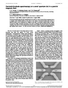
Keywords: generation capacity resource risk assessment, ABSTRACT The power density method for estimating potential power generation capacity is recommended for geothermal prospects at an exploration or early appraisal stage because it is relatively simple, case histories have been graphically compiled to support parameter estimates, and its pitfalls are more easily appreciated than is the case for most alternatives. In this implementation, a lognormal probability density function (PDF) for generation capacity in MW is obtained by multiplying two lognormal PDFs, one for interpreted resource area in km2 and one for power density in MW/km2. The PDF for the interpreted area of the resource is estimated by constructing a range of geothermal resource conceptual models called the P10, P50 and P90 models representative of the 10, 50 and 90 percentiles of the cumulative distribution function that are commonly used in resource assessment. The cumulative distribution function for power density can be estimated from the Wilmarth and Stimac graphical compilation of worldwide geothermal field power density versus resource temperature, categorized by conceptual setting. The resulting PDF for power generation capacity is typically expressed as 10, 50 and 90 percentiles of MW. The relative simplicity of the power density approach makes the recognition and mitigation of its pitfalls more manageable. For example, a commonly encountered pitfall is unrealistic area estimation. Many practitioners use the areas encompassed by different contour values of low resistivity “anomalies” to define the P10, P50 and P90 areas of a geothermal resource, a procedure that often produces unrealistically large resource capacity estimates. The recommended remedy is to base area estimates on geothermal resource conceptual models that integrate available geoscience data in a manner consistent with hydro-thermodynamics, with a range between the P10 and P90 estimates that considers both data and conceptual uncertainty. Ideally the estimates of power density from developed fields used to support this process would also be based on resource conceptual models. However, these are seldom available for an entire field outline, so developed field areas have been estimated from the perimeter of the drilled production wells. Inconsistencies in area and power density can be mitigated by checking for close analogies among the specific fields in the part of the Wilmarth and Stimac compilation that was used to estimate power density. This approach has been implemented in an Excel workbook that, as freeware, has been widely used for training courses and economic decision-making in the geothermal industry. Because standard Excel statistical functions can be used to represent and multiply lognormal PDFs, no Monte Carlo simulation is required. Besides the P10, P50, P90 and Mean MW, the spreadsheet provides the nu and sigma parameters representing the mean and variance of the logarithm of power generation used by software like @Risk ®Palisade and Crystal Ball®Oracle. To investigate the financial viability of a geothermal prospect assessed using the power density worksheet, the Excel workbook also includes a worksheet with a financial decision tree that considers five outcomes, exploration failure (no commercial production), appraisal failure (testing does not demonstrate minimum commercial size), and three development cases for power plant capacities that might plausibly be constructed. The probabilities for each branch of the decision tree are computed from the power capacity lognormal PDF and these are used to weight the net present value (NPV) and discounted investment (DI) that are separately provided for the five outcomes to provide expected NPV and DI for the prospect. The Excel Workbook sheet is available from the author as freeware, subject to users’ reference to this paper in initial publications of studies that utilize it. 1. INTRODUCTION The geothermal resource capacity estimation Excel workbook described in this paper is not new, having been used since 2000 to support exercises in courses and workshops on using geothermal resource conceptual models to assess resource capacity and its uncertainty at the exploration and early drilling appraisal stage of geothermal development. The concepts involved are also not new, with antecedents in geothermal (Grant and Bixley, 2011) and petroleum resource assessment (Schuyler and Newendorp, 2013). Although initially intended to be an educational illustration of geothermal resource capacity uncertainty and its economic consequences, the workbook has been widely used in the geothermal industry for prospect ranking and economic assessment prior to development, and so interest has grown in a publication on its use. The event that led me to prepare this paper is the publication by Wilmarth and Stimac (2015) of supporting information on trends in power density versus geothermal resource temperature and geological setting. Several geothermal developers have completed proprietary compilations but earlier publications tended to either emphasize the uncertainty in power density (Bertani, 2005) or to simply provide an overall average based on a limited sample (Grant and Bixley, 2011). The Wilmarth and Stimac compilation continues to evolve as illustrated in Figure 1 from Wilmarth et al. (2015). Beginning with Muffler (1979), variations on volumetric-heat-in-place estimation of geothermal resource capacity have dominated published approaches to capacity assessment prior to drilling. In the volumetric-heat-in-place approach, PDFs are estimated for the 1
Cumming resource area and thickness (volume), the resource temperature, and a recovery factor to obtain the probability distribution function for the “heat in place” that is recoverable for electrical generation, usually assuming that a variety of parameters are less uncertain and so can be reliably fixed, such as the rejection temperature and the efficiency of the conversion of heat to electrical generation. As noted by Grant and Bixley (2011), such methods have been used successfully but, as emphasized by Grant (2015), they can be easily manipulated to produce highly misleading results. Although all methods are susceptible to manipulation, the relative simplicity of the power density approach makes it easier to audit. It is based on the best constrained capacity-related parameters that are available for a large proportion of the world’s developed geothermal fields, their operating capacity in MW and their drilled area. Moreover, it is also based on the parameters of geothermal prospects that are best constrained by exploration data, the area, temperature and geological setting. If further information is available, perhaps thickness from a single borehole, then that can be considered by choosing a power density typical of specific fields with roughly analogous parameters. Ultimately all reliable methods for assessing resource capacity depend on analogy and I recommend the use of specific analogies as a check on statistical methods. In a geothermal context, a frequentist statistics approach is potentially more misleading than analogies because the number of developed geothermal fields is on the order of 100, rather than the 1000 to 10000 samples needed to produce reliable frequentist statistics. A general outline of the computation of a PDF for geothermal resource capacity from PDFs for power density and area introduces the functions and expressions used in the Excel worksheet and a summary of the supporting parameters. The lognormal PDF of resource generation capacity calculated in the first worksheet in the workbook is applied in a second worksheet that uses a decision tree to compile PDF weighted economic outcomes of the most plausible geothermal development capacities into an overall economic assessment of the resource. A review of the pitfalls of this approach and suggested remedies emphasizes the need for training that includes building geothermal resource conceptual models and practicing making realistic resource decisions.
Figure 1: Power density versus reservoir temperature categorized by geological setting. The pump exclusion zone refers to resources where temperature is too low for economic flash production for direct steam utilization but it is too hot for pumped production. Some wells within fields have flash production supporting binary generation in this gap. This figure and its use is explained in Wilmarth and Stimac (2015) and this version is from Wilmarth et al. (2015). 2. COMPUTING LOGNORMAL PDF PARAMETERS IN EXCEL FOR A RESOURCE CAPACITY WORKSHEET This Excel spreadsheet uses the built-in statistical functions of Excel to compute the parameters for the PDFs in a much simpler manner than approaches that use Monte Carlo simulation to approximate the product of several properties’ PDFs. As pointed out by Onur et al. (2010), the type of computation used by Excel is also more accurate, although this is a minor consideration given the much larger uncertainties in the input parameters. The parameters used in this spreadsheet, power density and area, are lognormally distributed (Wilmarth and Stimac, 2015). A parameter that is a product of two parameters with lognormal PDFs will also have a lognormal PDF, so the resource capacity computed using this spreadsheet has a lognormal PDF. 2
Cumming The most common approach in the geothermal and petroleum industries to specifying PDFs follows a resource practice where P10, P50 and P90 correspond to 10, 50 and 90 percentiles of the cumulative distribution function (e.g. Capen, 2001). This spreadsheet conforms to the usage where P10 is the optimistic case representing 10% confidence and P90 is the pessimistic case representing 90% confidence. This differs from the practice of many geothermal groups (and myself, much of the time), in which P10 is pessimistic based on the 10th percentile of the cumulative distribution and P90 is optimistic (Omer et al., 2010), but it is trivial to redefine the spreadsheet parameters to accommodate either practice. Because a lognormal PDF is completely specified by any two values of the parameter and their cumulative probabilities, then estimates of the P10 and P90 values of area can be used to define the variance and mean of the area PDF. The same confidence levels can be used to specify the power density PDF. From the variance and mean of the area and power density PDFs, the variance and mean of the PDF of the product of the two parameters can be computed, and from those, the P10, P50 and P90 estimates of power capacity. The equations for variance, mean and other characteristics of lognormal PDFs can be found in Onur et al. (2010) and many reference books. Because the focus of this paper is on the worksheet, the formulas are presented here using the Excel statistical functions, LOGNORMDIST, LOGINV and NORMSINV and the Excel mathematical expressions EXP and LN. Beginning with Excel 2010, new versions of the first three functions have been added, LORNORM.DIST, LOGNORM.INV and NORM.S.INV, respectively. These new functions include additional parameters not needed for this computation and so the older functions are used for backward compatibility. A user of the spreadsheet wanting to estimate a resource capacity distribution would estimate four parameters, values at two levels of confidence for area and two for power density. For example, based on pessimistic P90 and optimistic P10 conceptual models, estimates of the area in km2 at 90% and 10% confidence can be entered into spreadsheet cells named AreaP90 and AreaP10, respectively. AreaMean is the mean of the probability density function for Area. Estimates of spreadsheet cells PowerDensityP90 and PowerDensityP10 in MW/km2 could be estimated based on Figure 1, considering evidence for the temperature and geological setting of the area. For most users, these four parameters are the only ones required for the computation of the PowerCapacity probability density function in MW. LnAreaNu and LnAreaSigma are the mean and variance of LnArea in logarithmic units, respectively. LnAreaP10 =LN(AreaP10)
(1)
LnAreaNu =(LN(AreaP10)+LN(AreaP90))/2
(2)
LnAreaSigma =(LN(AreaP10) – LN(AreaP90))/(NORMSINV(0.9)-NORMSINV(0.1))
(3)
AreaMean=EXP(LnAreaNu+LnAreaSigma^2/2)
(4)
The following formula can be used to calculate the area at the confidence level of n in percent, AreaPn. AreaPn=LOGINV(1-n/100, LnAreaNu, LnAreaSigma)
(5)
AreaP99= LOGINV(0.99, LnAreaNu, LnAreaSigma)
(6)
For example,
This can be supplemented by the alternative expression for median, AreaP50=EXP(LnAreaNu)
(7)
Similarly, the mean and variance of the PDF for the logarithm of power density are LnPowerDensityNu and LnPowerDensitySigma, respectively, and can be similarly computed from the spreadsheet user’s estimate of PowerDensityP90 and PowerDensityP10. Because the equations can be derived from equations 1 to 7 by substituting the characters “PowerDensity” for “Area”, they are not shown. The mean and variance of the PDF for the logarithm of power capacity are LnPowerCapacityNu and LnPowerCapacitySigma, respectively, which are computed by the spreadsheet using the following formulas. LnPowerCapacityNu = LnAreaNu + LnPowerDensityNu
(8)
LnPowerCapacitySigma = (LnPowerDensitySigma^2 + LnAreaSigma^2)^0.5
(9)
From these values of the mean and variance of the PDF for the logarithm of power capacity, the power capacity at any confidence level n in percent can be estimated. PowerCapacityPn=LOGINV(1-n/100, LnPowerCapacityNu, LnPowerCapacitySigma)
(10)
For example, to estimate the optimistic P10 power capacity, the equation would be PowerCapacityP10= LOGINV(0.9, LnPowerCapacityNu, LnPowerCapacitySigma)
(11)
To compute ConfidenceXMW, the confidence (as a probability) that the power capacity will be greater than a capacity X in MW, ConfidenceXMW= (1-LOGNORMDIST(X, LnPowerCapacityNu, LnPowerCapacitySigma)) 3
(12)
Cumming
Figure 2: Spreadsheet for Geothermal Resource Capacity from Power Density. The upper block includes an initial assessment of the probability that the capacity distribution is valid, that is, that any potentially commercial geothermal resource exists, following petroleum practice of considering the existence of the essential elements of a resource separately from the resource capacity distribution, as defined in equation 1 to 11 above. Based on only the entries in the red outlined cells in Figure 2 of P10 and P90 values for area in km2 and power density in MWe/km2, equations 1 to 11 are used to compute the remaining area, power density and MWe capacity parameters in the worksheet. The nu and sigma variables are provided so that the worksheet PDFs can be easily used in decision assessment programs like @Risk®Palisade and Crystal Ball®Oracle. Besides the parameters used to compute the lognormal capacity distribution, the worksheet shown in Figure 2 includes red outlined cells for entries to support a separate estimate of the probability of exploration success (POSexpl) that is used to down-weight the capacity assessment. In most geothermal Monte Carlo heat-in-place assessments, only capacity is estimated. However, risk assessment experience in petroleum exploration has demonstrated that an approach that considers only the capacity PDF tends to bias estimates to represent the very small undeveloped reservoirs about which not much is known. As a ploy to focus experts on what they know, the POSexpl parameter is designed to exclude all reservoirs too small to be considered part of the experience of the experts. In a manner analogous to the POSexpl prerequisites often used in O&G assessments, like source rock, migration path, reservoir rock and trap (Schuyler and Newendorp, 2013), geothermal reservoir assessments commonly use prerequisite temperature, permeability and chemistry. A common metaphor used for this parameter is that it represents the probability that a plausible exploration program of 1 to 4 wells would encounter commercial productivity (in a conceptual sense) that meets the three prerequisites. The Ptemperature parameter is constrained most reliably by wells, gas and water geothermometry, active alteration/deposition of silica and evidence of heat loss. The Ppermeability parameter is constrained by confidence in the structural model and its interaction with formation properties and the chemistry of correlated leakage. The Pchemistry parameter is mainly directed at the implications of magmatic vapor-core like those drilled at Mt Apo, Alto Peak, Miravalles and other geothermal fields, mainly characterized by gas and water chemistry, sulfur deposition and active volcanic vents. The worksheet includes three cells outlined in red for optional entries. The cumulative probability of the optimistic case is set to the generally used standard of 10% but this can be adjusted. Some groups have concluded that, because they lack a sufficiently wide range of experience in geothermal assessment to support a P10 to P90 confidence interval, they are likely to underestimate variability. Therefore, they assume that their estimates represent a P20 to P80 confidence interval, with an entry of 20% as their cumulative confidence in their optimistic case. The temperature cells are not used in the computation but are intended to document the part of the Wilmarth and Stimac (2015) cross-plot that was used to estimate power density.
Figure 3: Spreadsheet for Geothermal Resource Capacity from Power Density. A risk tree indicating the computation of financial outcomes based on the resource parameters computed in the example shown in Figure 2. It commonly occurs that the P90 capacity estimate in Figure 2 is too small to be economic and the P10 capacity is unlikely to be constructed within the financial time line, perhaps due to a limited market size. Therefore, to provide an estimate of practical outcomes 4
Cumming and their financial implications, the workbook includes the five branch decision tree shown in Figure 3. It computes the probabilities of specific power plant developments that might be constructed based on the power capacity distribution in Figure 2 using equation 12. The net present value (NPV) and expected discounted investment (DI) for each power plant size as well as the NPV and DI for an exploration failure case (no commercial production) and an appraisal failure case (testing does not demonstrate minimum commercial size) are separately provided by a economics team. The probabilities for each branch of the decision tree are computed from the power capacity PDF and these are used to weight the NPV and DI of each branch to provide an expected NPV and DI for the prospect. 3. PITFALLS AND REMEDIES The most obvious objection to calculating capacity of exploration prospects using power density constrained by well perimeters as Wilmarth and Stimac (2015) have done is that exploration assessments of area are based on information like MT resistivity surveys or thermal manifestations, not on well perimeters. The area of low resistivity detected by an MT survey is not usually directly comparable to the area of the reservoir and is often several times larger. Using a particular data pattern like the area within a contour of particularly low resistivity to assess resource area or target wells is called anomaly hunting or data targeting. This approach works by direct analogy and it is cost-effective for low value decisions. For high value decisions like capacity estimation or well targeting, this approach is unreliable. Modern publications on best practices in the geothermal industry emphasize the use of geothermal resource conceptual models in such assessments (e.g. IGA Service GmbH, 2014; US-DOE, 2014). Cumming (2016) provides a step-by-step tutorial on building a suitable range of P10, P50 and P90 resource conceptual models for a volcanic geothermal prospect based on geochemistry integrated with geology, and MT resistivity, together with a summary of pitfalls and remedies. As part of an explanation of a strategy for exploring for “blind” geothermal prospects, Cumming (2009) summarizes a conceptual model for a sediment-hosted geothermal reservoir. Ideally the estimates of power density from developed fields used to support this process would also be based on resource conceptual models. However, these are seldom available for an entire field outline, so developed field areas have been estimated from the perimeter of the drilled production wells. Inconsistencies in area and power density can be mitigated by checking for close analogies among the specific fields in the part of the Wilmarth and Stimac compilation that was used to estimate power density. In addition to using specific analogies to check the plausibility of assessments made using a power density approach, I recommend results to whatever alternative methods seem relevant, including any Monte Carlo heat-in-place estimates that may be available. If tested wells are available, more elaborate approaches like stochastic reservoir simulation can be used to independently assess capacity and its uncertainty (Parini and Riedel, 2000). Supporting strategies commonly include using decision tables to organize and document parameter choices, with the POSexpl and P10, P50, P90 parameters as column headings, the different conceptual models and data types as row headings and the cells including brief summaries of the influence of the data in the rows on the parameters in the columns. Because the limited number of developed geothermal fields does not support the use of population statistics in geothermal resource capacity assessment, the problem is more amenable to a Bayesian view of the available evidence (Hastie et al., 2008). However, more explicit Bayesian estimation of a prior probability that is updated based on new information complicates the assessment process in ways many people find non-intuitive. For example, it is difficult to estimate what opportunities are implied by the lack of information about prospects that do not support assessment using conventional exploration geochemistry indicators (the so-called “hidden” or “blind” prospects). An analysis of such a case tends to result in a conclusion that, if the chemistry of thermal manifestations is uninformative, then low cost wells are needed to provide information about potentially commercial temperature, ideally including fluid chemistry but at least a thermal gradient in a potential resource cap. If drilling a suitable gradient well is uneconomic, the prospect is probably too risky but, if drilling is feasible, then a conventional risk assessment will also be feasible. Nonetheless, the conceptual implications of Bayesian confidence estimation rather than estimation based on fictitious population distributions are useful, especially as geothermal exploration is increasingly directed at prospects that are partially “hidden” or otherwise do not fit the conventional geothermal exploration paradigm. A frequently advertised alternative strategy to assess resource capacity or target wells that avoids the need to build conceptual models is to compile all available data for a group of geothermal fields and prospects, compute a statistical predictor using training data sets at the existing fields, and then using that predictor to assess the area, capacity or targets at new prospects. This is superficially appealing because it appears to more effectively employ under-utilized data and can be done by the statisticians without highly specialized expertise in the thermodynamic and geoscience properties of geothermal fields. The problem has been that, providing that a large enough number of data sets is provided, the method always works in that it always “predicts” the existing field parameters but its success in predicting new areas is very unreliable. This is due to well-known predictive modeling fallacies, illustrated by spectacular failures in the financial industry (Silver, 2012). These methods highlight a general misimpression that using more data and/or more types of data will always result in better decisions. Assessing what data has the best predictive performance for resource capacity and well targeting is further complicated by the bias in reporting successes but not failures. One of the advantages of using a conceptual model approach supported by case histories is that it provides an organizing principal for prioritizing conventional data sets and a guide to how new types of data are likely to improve the reliability of well targeting and resource capacity assessments, analogous to the “Take the Best” heuristic in decision theory (Gigerenzer and Goldstein, 1997). A common procedural pitfall in utilizing power density (or any capacity assessment approach) is to provide a group of qualified experts a cursory review of a prospect and then ask them to vote on the probability of success and the P10, P50 and P90 values based on their limited information. When there is a disparity of information among experts, voting is usually a poor choice, except for quick, low value decisions. In cases where the presenters are much more familiar with the resource issues, conducting a peer review by outside experts to ensure, for example, that a representative range of analogous case histories have been considered, will usually be more effective than simply voting. If time is not available for a peer review, it is usually better to emphasize the opinions of the best informed, another variation on the “Take the Best” heuristic. However, perhaps the greatest challenge in utilizing expert opinion in the boom phase of the 5
Cumming boom-and-bust geothermal industry has been finding a quorum of experts who have sufficiently broad geothermal experience to support a peer review of resource conceptual models and their uncertainty. In order to reliably support resource assessment using this power density approach, geothermal geoscientists need practice building conceptual models, predicting resource capacity and well targets, and reviewing their prediction performance (Silver, 2011). To understand the minimum likely range of models, they will also require familiarity with a wide range of geothermal conceptual models and their supporting evidence. However, with fewer than 100 geothermal fields developed over the last 50 years, few geothermal exploration staff have had sufficient career experience to appreciate the uncertainty of capacity assessment or the risks of exploration drilling. Most geothermal geoscientists are familiar with only a few geothermal fields and prospects, perhaps just those operated by their employer, and most researchers have only a very narrow conceptual understanding of geothermal systems relevant to the own research interest. Although geothermal geoscientists should make reviewing potentially analogous geothermal conceptual case histories a routine part of their assessments, this does not provide practice in making and testing geothermal resource predictions. One remedy for this is to train geothermal management and geoscience staff using simulations of geothermal conceptual model development, capacity estimation and well targeting based on case histories of developed geothermal fields. 4. CONCLUSIONS An Excel spreadsheet is available from the author that uses the built-in statistical functions of Excel to compute resource capacity uncertainty based on the power density method and the lognormal PDFs that are appropriate for such parameters. The simplicity of this approach supports straightforward documentation using decision tables and easier auditing. Common pitfalls such as estimating areas from resistivity anomalies or the perimeter of thermal manifestations can be addressed by estimating area from a range of integrated resource conceptual models representative of the P10, P50 and P90 areas used in the capacity assessment. Wilmarth and Stimac (2015) provide support for estimating power density based on developed geothermal reservoirs with analogous temperature and geologic setting. The most serious pitfall in the use of this approach is its implicit requirement of expert experience. More reliable results are expected from users who have experience in building resource conceptual models, broad knowledge of a suitable range of geothermal resource case histories, and routine practice in predicting resource capacity and testing the reliability of predictions against outcomes. Very few geothermal geoscientists worldwide have such experience. To address this, the professional development of geothermal geoscientists should include an explicit investment in learning case histories analogous to their area of work and in synthesizing experience in assessing geothermal exploration and development decision risk issues and testing prediction performance, potentially through exploration and development scenario workshops based on actual case histories. REFERENCES Benoit, D.: An Empirical Injection Limitation in Fault-Hosted Basin and Range Geothermal Systems, Geothermal Resource Council Transactions, 37, (2013), 887-894. Bertani, R.: World Geothermal Power Generation in the Period 2001–2005, Geothermics 34 (2005), 651–690. Capen, E.: Probabilistic Reserves! Here at Last?, SPE Reservoir Evaluation & Engineering, (2001), 387-394. Cumming, W.: Geothermal Resource Conceptual Models Using Surface Exploration Data, Proceedings, 34th Workshop on Geothermal Reservoir Engineering, Stanford University, Stanford, CA (2009). Cumming, W.: Resource Conceptual Models of Volcano-Hosted Geothermal Reservoirs for Exploration Well Targeting and Resource Capacity Assessment: Construction, Pitfalls and Remedies, Geothermal Resources Council Transactions 40 (2016). Garg, S. and Combs, J.: A Reexamination Of USGS Volumetric “Heat In Place” Method, Proceedings, 36th Workshop on Geothermal Reservoir Engineering, Stanford University, Stanford, CA (2011). Grant, M. and Bixley, P.: Geothermal Reservoir Engineering 2nd Edition, Elsevier, Amsterdam, (2011), 359. Grant. M.: Resource assessment, a review, with reference to the Australian Code, Proceedings, World Geothermal Congress, Melbourne, Australia (2015). Hastie, T., Tibshirani, R., Friedman, J.: The Elements of Statistical Learning, Data Mining, Inference, and Prediction 2nd Edition. Springer Series in Statistics, (2008), 745. IGA Service GmbH: Best Practice Guide for Geothermal Exploration. Report written by GeothermEx Inc for International Finance Corporation, edited by Dr. Colin Harvey for IGA Service GmbH. (2014),196 pp. Gigerenzer, G. and Goldstein, D.: Reasoning the fast and frugal way: Models of bounded rationality, Psychological Review 103 (1996), 650-669. Muffler, P.: Assessment of geothermal resources of the United States -1978, USGS circular 790, (1979), 164. Onur, M,. Sarak, H., and Türeyen, Ö.: Probabilistic Resource Estimation of Stored and Recoverable Thermal Energy for Geothermal Systems by Volumetric Methods, Proceedings, World Geothermal Congress, Bali, Indonesia (2010). Parini, M. and Riedel, K.: Combining probabilistic volumetric and numerical simulation approaches to improve estimates of geothermal resource capacity, Proceedings, World Geothermal Congress, Tokyo, Japan (2000). 6
Cumming Sanyal, S. and Sarmiento, Z.: Booking Geothermal Energy Reserves, Geothermal Resources Council Transactions 29 (2005), 467-474. Schuyler, J., and Newendorp P.: Decision Analysis for Petroleum Exploration, 3nd Edition, Planning Press. (2013), 588. Silver, N.: The signal and the noise: Why so many predictions fail--but some don't. Penguin Books. (2012), 560. US-DOE: Best practices for Risk Reduction Workshop Follow-up Manual. Published 8-Jul-2014. (2014), 40. Wilmarth, M. and Stimac, J.: Power Density in Geothermal Fields, Proceedings, World Geothermal Congress, Melbourne, Australia (2015). Wilmarth, M., Sewell, S. and Cumming, W.: Resistivity imaging and interpretation strategies to reduce uncertainty in geothermal resource capacity estimation. Fall Meeting, American Geophysical Union, San Francisco (2015).
7