shape of the parallelism curve is characteristic of the form of the source code shown below. The source code is developed in the SISAL language. [2], and has ...
Multiprocessor Resource Estimation Using a Stochastic Modeling Approach D. L. Andrews, M. A. Thornton, J. D. Bullard Department of Computer Systems Engineering University of Arkansas
Abstract A modeling approach based upon the notions of thread spawning and maximum length probability density functions is presented. By using a data dependence graph, or alternatively, an available parallelism profile, probability density functions may be derived and used as input to a queuing system model that can predict required resources.. The accuracy of the model is measured by validation using parallelism profiles under different halting criteria. The result of this work is the establishment of a modeling framework that can later be used to estimate the effects of non-zero interprocessor latencies and limitations due to a finite number of processing elements.
1 Introduction Parallelism profiles have been used in the past to evaluate the available parallelism contained within an application program. These parallelism profiles show the number of parallel operations available at each step of program execution. This paper presents a model derived from parallelism profiles for analyzing the overhead associated with the creation and completion of parallel operations. The model presents a method for determining the overhead associated with executing the program. This information can be used to determine the granularity of parallel operations within a program, partitioning, and load balancing, or determining optimal thread sizes for multithreaded architectures. Unfortunately, parallelism profiles only give the upper bound in achievable parallelism for a given architecture. Multiprocessor designers typically must specify a system and simulate different programs to determine the behavior of the architecture which is then compared against the ideal case given in the parallelism plot. In this work, we define several parameters that are directly measurable from the parallelism plots and develop a statistical queuing model for execution of the program. Since the
model can be used to generate ideal cases, it is validated by comparing it against the original ideal data. Most queuing models for multiprocessor systems only predict steady state responses by ignoring start-up and shut-down transients since they are typically too hard to model. In this work, we include the transients in the model through the notions of maximal thread length and thread spawning probability density functions (pdf). The pdfs are generated directly from the available parallelism curves and are used to pseudo-randomly generate random variables that represent the initiation and duration of maximal length computation threads. The halting criteria proved to be a major parameter with regard to the accuracy of the model. We report the results of three different halting criteria. We have determined that the best halting criteria is to equate the amount of work present in the available parallelism curve to that predicted by the simulation. When the maximum work criteria is used, acceptable estimates of total runtime and maximum required processing elements are predicted when compared to the ideal case. This validates the approach for estimating the results of non-zero latencies or restricting the number of available processing elements in other experiments using the model. The next section contains a review of the available parallelism plots and provides a brief explanation of their significance and origin. In section 3 we define various parameters that are computed from the available parallelism plots and used as inputs to the statistical model. Section 2 contains a description of the model and experimental results using several benchmark cases. Finally, the results of this work and areas of future related effort are outlined in the conclusion section.
2 Parallelism Profiles Parallelism profiles present a graphical representation of the parallel operations available for execution at each time step in a program. A typical parallelism profile is
Loop 11 Parallelism 300
Parallelism
250 200 150 100 50 0 0
4
8 12 16 20 24 28 32 36 40 44 48 52 56 60 64 Tim e
Figure 1. Parallelism Profile for Livermore Loop 11. shown in Figure 1. This parallelism profile taken from Loop 11 of the Livermore Loops [1] [5] shows the number of parallel operations available for execution at each time step in the program. The parallelism profile shows that a variable number of operations are available for execution in parallel throughout the lifetime of the program. The shape of the parallelism curve is characteristic of the form of the source code shown below. The source code is developed in the SISAL language [2], and has been modified from the original iterative FORTRAN source code. The modification uses recursive doubling and is more efficient for parallel execution than the original FORTRAN source code. The modified code is shown in Figure 2. This transformation executes in O(log n) in time, and O(n log n) in number of operations [1]. % Loop 11 - First Sum % function Loop11(n:integer; Y:OneDim; returns OneDim) for initial i := 1; X := Y while i < n repeat i := 2*old i; X := array_adjust(old X, 1, old i) || for j in old i+1, n returns array of old X[j] + old X[j old i] end for returns value of X end for
end function %Loop11 Figure 2. SISAL Code for Livermore Loop 11 The envelope of the curve is determined by the inner parallel For construct, and the number of spikes shown in Figure 1 is determined by the outer while loop. For a detailed discussion of the Livermore Loops, see [1]. The parallelism profile provides insight into the architectural characteristics of the machine type best suited for executing the program. The maximum number of processors required in order to exploit the parallelism can easily be determined by analysis of the profile graph. The maximum number of parallel operations and hence, the maximum number of processors required for this profile is 250. The area under the parallelism profile represents the total work required to execute this program.
3 Source/Sink Thread Overhead One factor that will affect the execution time of the program is the overhead associated with task creation, completion, data copying, synchronization, etc., as well as resource contentions associated with the initialization and termination of the parallel operations. The effects of this overhead is not apparent by the data displayed in the parallelism profile. The parallelism profile is based on a data dependence ordering of operations by level. The parallelism profile shows the cumulative number of operations at each level, but does not show actual execution times.
A model can be developed based on the parallelism profile to aid in the understanding of the overhead of creating and executing these parallel operations. The model is based on the following definitions: Maximal Process Thread: All Instructions are executed on a single processing element. Maximal Source Overhead: The overhead associated with starting execution of a new maximal thread . Maximal Sink Overhead: The overhead associated with terminating a maximal thread. Average Maximal Thread Length: The average number of operations maximal threads.
executed in all
The first graph in Figure 3 shows a data dependence graphical representation of a single thread. The data graph provides a strict ordering of operations represented by the data dependencies between the operations in the graph. The single thread shown in Figure 3 contains a single sequential ordering of operations. The second graph in Figure 3 shows three new threads sourced from the top most node. Overhead will be introduced when these three threads are sourced. This overhead can be attributed to operating system scheduling, resource deallocation and contention, or transfer of data. The third graph in Figure 3 shows three threads that will be terminated by transferring data into the thread that contains the bottom node. Overhead will also be introduced when these three threads are sinked. It is apparent from the second and third graphs shown in Figure 3 that exactly three threads are sourced, and three are sinked. This level of detail cannot be accurately obtained from a parallelism profile. Each time step shown in a profile shows the net number of parallel operations existing at that level. Consider the parallelism profile
shown in Figure 1. The profile shows approximately 120 parallel operations exist at time step three, and 250 parallel operations exist at time step four. A net of 130 new parallel operations were sourced between time step three and four. However, the profile does not provide enough information to determine if 130 new operations were sourced, or if the 120 operations in time step three were sinked, while 250 new operations were sourced. This information is available from the source program, or the data dependence graph, but not the parallelism profile. The following definitions are required to continue definition of a model based on the parallelism profile. Let N(t) ≡ number of processors required at time t in the parallelism profile. Enumerate PEi = i ∀i ∈ [1,n] where n is the maximum number of processors required throughout the program execution. For the parallelism profile illustrated in Figure 1, the value of n = 250. If N(t) = k, then PE1, PE2, . . . PEk are executing, and PEk+1 . . . PEn are idle. If N(t+1) > N(t), then we assume processors PEN(t+1) . . . PEN(t)+1 initiate execution. Processors PE1 . . . PEN(t) continue execution, assuming N(t) ≤ n. If N(t+1) < N(t), then we assume processors PEN(t+1)+1 . . . PEN(t) terminate execution. Processors PE1 . . . PEN(t+1) continue execution. A maximal process thread is defined to operate on processor PEk over the time interval [α,β], with length β − α, such that k ≥ N(t) ∀t ∈ [α,β]. The following two observations are a direct result of this Lemma: Lemma 1: The maximal process thread of PEi ≥ PEi+1. PROOF: The maximal process thread of PE1 is exactly equal to the critical path, and hence, the overall depth of the data dependence graph. This corresponds to the overall execution time of the program. QED
1 T h re ad
T hr e a d 1
op
op
Threa d 2
T hr e a d 3
op
op
op
op
op
op
op
op
3 T h r ea d s s ou rce d
op
op
op
op
T h rea d 4
op
op op
op
op
op 3 T hr e ad s si nk ed
R e su lt
T h re a d 1
T hr e a d 2
T hr e a d 3
op
T h rea d 4
Figure 3. Thread Definitions
3.1 Source/Sink Definitions We define ∆N(t ) as: ∆ fN(t ) = N(t + 1) − N(t )
∆ bN(t) = N(t) − N(t − 1)
where ∆ fN(t ) is a first order forward difference equation, and ∆ bN(t) is a first order backward difference equation [3]. ∆ fN (t ) represents the net number of maximal threads spawned, and ∆ bN ( t ) represents the net number of maximal threads sinked at time t. Define Src(t) and Snk(t) as: 1 [| ∆b N(t) | +∆b N(t )] 2 1 Snk (t) = [| ∆fN (t) | − ∆fN(t )] 2 Src (t) =
Src(t) represents the number of maximal threads sourced, and Snk(t) represents the number of maximal threads sinked at time t. For any program ∞
∑
0 ≤ Src(t) ≤ max | ∆ fN(t ) | 0 ≤ Snk(t) ≤ max | ∆ bN(t) | , max | ∆ fN (t ) | , max | ∆ bN ( t ) | ≤
The graph shown in Figure 4 illustrates the Src(t) curve for the parallelism profile shown in Figure 1.
3.3 Probability Density and Distributions Define two random variables X and Y. We can define the event Ax to the subset of Src consisting of all sample points Src(t) to which the random variable X assigns the value x, and the event By to the subset of Snk consisting of all sample points Snk(t) to which the random variable Y assigns the value y [6]: Ax = {Src(t ) ∈ Src | X (Src ( t)) = x } By = {Snk (t) ∈Snk | Y ( Snk (t )) = y }
Using these definitions,
Src(t ) = # maximal length threads
t =1
∞
= ∑ Snk (t ) t=1
The number of maximal length threads sourced must equal the number sinked, otherwise, the program would not terminate. Based on the definitions for Src(t) and Snk(t), several observations can be made regarding the programs’ overhead behavior.
max | N ( t ) |
P(Ax) = P([X = x]) P(BY) = P([Y = y]) = P({Src(t) | X(Src(t)) = x}) P({Snk(t) | Y(Snk(t)) = y}) =
∑ P( S ∑ P( S
rc (t ))
X ( Src (t )) = x
=
nk (t ))
Y ( Snk( t )) = y
=
We define these functions as the spawning and sinking probability density functions (pdf), respectively. The following properties hold: 0 ≤ p(Src (t)) ≤ 1 P (Src ( t)) = 1
∑
x∈S rc
0 ≤ p(Snk (t )) ≤ 1 P( Snk (t)) = 1
FX(x) = P{X < x } = ΣfX(xi) FY(y) = P{Y < y } = ΣfY(yi) The spawning mass function represents the probability of spawning Src(t) new maximal threads during the execution of the program. The sinking mass function represents the
∑
y∈S nk
and the cumulative spawning and sinking distribution functions FX(x) and FY(y) as
Normalized Spawns
Spaw ns 140 120 100 80 60 40 20 0 0 3 6 9 12 15 18 21 24 27 30 33 36 39 42 45 48 51 54 57 60 63 Tim e
Figure 4. Src(t) Graph for Loop 11. probability of sinking Snk(t) maximal threads during the execution of the program. The spawning and sinking probability mass functions for the parallelism profile shown in Figure 1 are shown below in Figure 5. The cumulative normalized spawning density function shows that threads are spawned fairly uniformly throughout the life of the program. The cumulative normalized sinks density function shows that threads are terminated fairly uniformly throughout the life of the program. The distribution functions show the normalized number of spawns and sinks during execution. The distribution functions in Figure 6 show the number of spawns and sinks are fairly constant throughout the program.
3.4 Thread Length Density / Distributions The spawning and sinking density functions provide a technique to model the frequency of maximal thread creation and completion. This provides a measure of how active the program is during execution, and how the overhead of creation and completion is distributed
throughout the program. This cost of the overhead can be modeled by density and distribution functions of the length of the maximal threads. For long threads, the overhead cost is easily amortized over the length of the thread. This is typical of MIMD operation, where the length of the thread is long. For short threads, the overhead cost is not readily available, and can represent a significant delay in the thread execution. Short thread lengths are characteristic of SIMD operations. We define the random variable Z that maps the length of the maximal length threads to the real numbers. We define the event Ax to the subset of Src consisting of all sample points Src(t) to which the random variable X assigns the value x, and the event By to the subset of Snk consisting of all sample points Snk(t) to which the random variable Y assigns the value y: Ax = {Src(t ) ∈ Src | X(Src (t)) = x } By = {Snk (t) ∈Snk | Y(Snk (t )) = y }
Spaw ning D ensity
Probability
0.6 0.5 0.4 0.3 0.2 0.1 121
125
130
123
125
130
120
119
116
115
106
95
91
65
56
2
1
0
0
N um ber to Spaw n
121
120
118
115
108
95
93
65
58
3
0.8 0.7 0.6 0.5 0.4 0.3 0.2 0.1 0 0
Probability
S inking D ensity
N um ber to S ink
Figure 5. Density Functions
3.5 Overhead Granularity
4 Model Formulation
The parallelism profile in Figure 1 shows a large degree of parallelism is available periodically throughout the program. A total of 9000 threads are spawned during the programs execution. The average thread length is an important characteristic of the program, and can be determined by:
To investigate the validity of using spawning and thread length distribution density functions for characterizing exploitable parallelism in a given computer architecture, a statistical model was developed and run using the SIMSCRIPT simulation language [4]. The model consisted of a set of resources representing maximal length threads and two main processes; a GENERATOR and PE process. The GENERATOR process is responsible for randomly determining if and how many maximal length threads are spawned at each CPU clock cycle. The PE process represents a single processing element upon which a maximal length thread will execute. The PE process pseudo-randomly generates the length of a maximal thread by using a user defined probability density function. Likewise, the GENERATOR process determines the number of maximal length threads to spawn at a given time based upon another user defined probability density function.
threadlength =
1 # threads
∑t
i
i
where ti is the length of thread I. The thread length can also be computed by dividing the total area under the parallelism profile curve by the total number of threads. The average thread length for Figure 1 is 3.6. This implies only 3.6 instructions are executed on average in each thread.
The model also has the capability to add additional parameters such as latencies due to processing element overhead, and, to limit the number of available processing elements to some finite number.
125
130
125
130
121
120
119
116
115
106
95
91
65
56
2
1
1 0.9 0.8 0.7 0.6 0.5 0.4 0.3 0.2 0.1 0 0
Probability
Spawning Distribution
Number to Spawn
123
121
120
118
115
108
95
93
65
58
3
1 0.9 0.8 0.7 0.6 0.5 0.4 0.3 0.2 0.1 0 0
Probability
Sinking Distribution
Number to Sink
Figure 6. Distribution Functions
4.1Model Validation The accuracy of the model was tested by performing a series of runs using maximal thread spawn and length pdfs derived from the Livermore Loops and by using an unlimited number of processing elements with zero latency incurred. These parameters match the deterministic parallelism curves given in [1]. One additional parameter which is very important and crucial to the outcome of the model results is the number of initial threads executing. Upon examination of the deterministic data in [1], code segments such as the one represented by loop 10 begin with a small number of threads (less than 10) and at time 1 spawn several thousand threads (over 5500). We experimented with three different criteria for ending the simulation:
1. Halting when the absence of executing or queued threads is detected. 2. Halting when the amount of simulation execution time equals the total required time in the available parallelism plot. 3. Halting when the amount of work (measured in PE CPU cycles) in the simulation equals that in the available parallelism profile.
4.2 Experimental Results Table 1 contains results when the model halted as soon as no threads were executing, or waiting to be executed. Not surprisingly, the runtimes between the statistical
model and correlation.
the
parallelism
profiles
indicated
no
This is due to the fact that the threads are “spawned” randomly and in many cases the small initial number of threads finished execution before more threads were
generated. However, resource estimates were encouraging for several cases with the percent error less than 10%. Table 2 contains the comparison of the predicted resources versus the actual data derived from parallelism plots when the simulation was run for an amount of time equivalent to that in the profiles.
Table 1: Model Validation Results Using the Idle PEs Halting Criteria Loop 1 2 3 4 5 6 8 9 10 11 12 15 16 22 23
Execution Time Model Actual % Error 22 8 175% 28 109 74% 11 4 175% 21 19 11% 57 78 27% 21 635 97% 190 18 955% 41 14 193% 41 12 242% 72 65 11% 13 6 117% 523 25 199% 478 45 962% 149 12 114% 167 2030 112%
Average Number of PEs Model Actual % Error 1316.0 1493.8 12% 7.9 15.0 47% 1167.2 1250.0 7% 6.2 7.2 14% 122.0 117.3 4% 18.0 26.2 31% 706.9 822.0 14% 117.5 189.5 38% 1493.2 2228.3 33% 42.7 71.5 40% 1019.2 1000.2 2% 1062.8 1126.0 6% 104.3 156.3 33% 102.5 116.9 12% 130.9 23.5 457%
Maximum Number of PEs Model Actual % Error 2903 2950 2% 35 200 83% 1930 2000 4% 15 30 100% 374 500 25% 58 190 69% 2955 2975 1% 702 1000 30% 5352 5500 3% 129 254 49% 1877 2000 6% 3881 3290 18% 794 900 12% 237 200 16% 710 700 1%
5 Conclusion Table 3 contains the results when the halting criteria is set to equivalent amounts of work in the stochastic simulation and the available parallelism profiles. The best results are those that use the total work halting criteria. In roughly half of the benchmark cases the percent error is less than or equal to 5% in terms of resource estimation (required number of processing elements) and is greater than 15% in only 3 of the above 15 cases. Since the pdfs may be derived from data dependency graphs as well as available parallelism curves, the model may be used to estimate the required number of processing elements for a given data dependency graph.
We have developed a statistical model that can be used to predict needed resources for a parallel architecture based upon the notions of maximal length thread spawning and length probability density functions. This information is easily obtainable from available parallelism profiles or, data dependence graphs. The model was validated through comparisons to actual data and several different halting criteria were evaluated.
Table 2: Model Validation Results Using the Constant Run Time Halting Criteria Loop 1 2 3 4 5 6 8 9 10 11 12 15 16 22 23
Average Number of PEs Model Actual % Error 1373.3 1493.8 8% 2.6 15.0 83% 1321.2 1250.0 6% 4.8 7.2 33% 57.0 117.3 51% 1.1 26.2 96% 675.4 822.0 18% 122.1 189.5 36% 1580.3 2228.3 29% 24.0 71.5 66% 1103.4 1000.2 10% 1146.6 1126.0 2% 85.1 156.3 46% 100.5 116.9 14% 5.7 23.5 76%
Maximum Number of PEs Model Actual % Error 2471 2950 16% 33.2 200 83% 1839 2000 8% 15 30 50% 366 500 27% 60 190 68% 2031 2975 32% 510 1000 49% 3836 5500 30% 122.1 254 52% 1768 2000 12% 2996 3290 9% 447 900 50% 189 200 6% 708 700 1%
Table 3: Model Validation Results Using the Total Work Halting Criteria Loop 1 2 3 4 5 6 8 9 10 11 12 15 16 22 23
Execution Time Model Actual % Error 11 8 38% 110 109 1% 6 4 50% 22 19 16% 107 78 37% 967 635 52% 30 18 67% 26 14 86% 18 12 50% 94 65 45% 8 6 33% 35 25 40% 74 45 64% 21 12 75% 1969 2030 3%
Average Number of PEs Model Actual % Error 1740.2 1493.8 16% 22.4 15.0 49% 1467.1 1250.0 17% 10.1 7.2 40% 136.4 117.3 16% 27.0 26.2 31% 837.8 822.0 2% 255.2 189.5 35% 2718.7 2228.3 22% 78.2 71.5 9% 1380.6 1000.2 38% 1206.8 1126.0 7% 149.1 156.3 5% 110.4 116.9 6% 28.1 23.5 19%
The utility of this approach lies in the fact that parameters such as processor latencies and finite resources may be varied and the corresponding characteristics of a parallel architecture may be observed before high level design occurs. Thus, this tool can be valuable for the system designer in the specification phase of the processor architecture. Since the pdfs can be computed directly from a data dependency graph produced by a compiler, this model can be used to predict the required number of processing elements before the program is actually executed.
Maximum Number of PEs Model Actual % Error 3158 2950 7% 165 200 18% 2080 2000 4% 24 30 20% 486 500 3% 168 190 12% 2584 2975 13% 1103 1000 10% 6716 5500 22% 254 254 0% 2091 2000 5% 3173 3290 4% 883 900 2% 210 200 5% 776 700 11%
Bibliography [1] John. T. Feo, “An Analysis of the Computational and parallel complexity of the Livermore Loops” Elsevier Science Publishers B.V., Series on Parallel Computing 0167-8191/88, #7, 1988. [2] J. McGraw, S. Skedzielewski, R. Oldehoeft, J. Glauert, C. Kirkham, B. Noyce, R. Thomas, “SISAL Streams and Iteration in a Single Assignment Language” Language
Reference Manual, Version 1.2, M-146 Rev. 1 University of California-Davis, March 1985. [3] M.L. James, G.M. Smith, J.C. Wolford, “Applied Numerical Methods For Digital Computation”, Harper Row, 2nd ed. 1977. [4] E. C. Russell, SIMSCRIPT II.5 Programming Language, 4-th Edition, CACI Products Company, LaJolla, CA, 1987. [5] John T. Feo, “The Livermore Loops in SISAL”, Technical Report, UCID-21159, Lawrence Livermore National Laboratory, August 1987. [6] Kishor Trivedi, “Probability and Statistics with Reliability, Queuing, and Computer Science Applications”, Prentice Hall, 1982.