Resource Estimation in Software Engineering - Semantic Scholar

Resource Estimation in Software Engineering Lionel C. Briand Carleton University Systems and Computer Engineering Dept. Ottawa, ON K1S 5B6 Canada [email protected] Isabella Wieczorek Fraunhofer Institute for Experimental Software Engineering (IESE) Sauerwiesen 6 67661 Kaiserslautern [email protected]

International Software Engineering Research Network, Technical Report

ISERN 00-05

1

Resource Estimation in Software Engineering Lionel C. Briand and Isabella Wieczorek

1 Introduction This paper presents a comprehensive overview of the state of the art in software resource estimation. We describe common estimation methods and also provide an evaluation framework to systematically compare and assess alternative estimation methods. Though we have tried to be as precise and objective as possible, it is inevitable that such a comparison exercise be somewhat subjective. We however, provide as much information as possible, so that the reader can form his or her own opinion on the methods to employ. We also discuss the applications of such estimation methods and provide practical guidelines. Understanding this article does not require any specific expertise in resource estimation or quantitative modeling. However, certain method descriptions are brief and the level of understanding that can be expected from such a text depends, to a certain extent, upon the reader’s knowledge. Our objective is to provide the reader with a comprehension of existing software resource estimation methods as well as with the tools to reason about estimation methods and how they relate to the reader’s problems. Section 2 briefly describes the problems at hand, the history and the current status of resource estimation in software engineering research and practice. Section 3 provides a comprehensive, though certainly not complete, overview of resource estimation methods. Project sizing, an important issue related to resource estimation, is then discussed in Section 4. Section 5 defines an evaluation framework that allows us to make systematic and justified comparisons in Section 6. Section 7 provides guidelines regarding the selection of appropriate estimation methods, in a given context. Section 8 describes typical scenarios for using resource estimation methods, thereby relating them to software management practice. Section 9 attempts to define important research and practice directions, requiring the collaboration of academia and industry. Section 10 then concludes this article by summarizing the main points made throughout the article.

2 Resource Estimation in Software Engineering This section briefly summarizes current practices regarding resource estimation in software engineering. This will shed light on the importance of the research being conducted and presented in subsequent sections. 2.1

Current Practices and Motivations

The estimation of resource expenditures (e.g., effort, schedule) is an essential software project management activity. Inaccuracies in such estimations have repeatedly shown to lead to disasters (Heemstra, 1992). Delivering software on-time and within budget is a critical concern for organizations as underestimating software projects can have detrimental effects on business reputation, competitiveness, and performance (Putnam and Myers 1992; Lederer and Prasad, 1993). On the other hand, overestimated projects can result in poor resource allocation and

ISERN 00-05

2

missed opportunities to take on other projects. Industry has recognized that by improving project estimation methods, problems with resource allocation and schedule forecasting can be overcome (Heemstra, 1992). Project managers commonly stress the importance of improving estimation accuracy and methods to support better estimates (Lederer et al., 1990, Lederer and Prasad, 1992). Accurate estimates are crucial for better project planning, tracking, and control and pave the way for successful project delivery. Software resource estimation is considered to be more difficult than resource estimation in other industries. Software organizations typically develop new products as opposed to fabricate the same product over and over again. This leads to many difficulties in estimating the resources of a project, especially in early project phases. Many studies have confirmed that a majority of projects overrun their budget (e.g., Jenkins et al., 1984; Heemstra, 1992; Lederer and Prasad, 1992; Lederer and Prasad, 1995). Practitioners are often faced with the lack of explicit cost and resource data collected from past projects (Heemstra, 1992). Moreover, estimators rely more on their personal memory and informal procedures than on documented facts, standards, or arithmetic rules (Hihn, 1991; Lederer and Prasad, 1992). Hence, estimates based on expert judgement and based on the available capacity prove to be quite popular (Heemstra, 1992). If actual data was recorded than only little time is spent to determine reasons for any difference between actual and plan data (van Genuchten, 1991). Many commercial packages are available on the market and one might be tempted to use some of them. However, experience has shown that one should not rely on software estimation tools for an accurate estimate, i.e., no difference was found between organizations using the tools and those not using the tools in terms of accuracy (Lederer and Prasad, 1992). The difficulties in software estimation are related to a variety of practical, measurement, and modeling issues. To address these issues, it is necessary to follow a systematic estimation process that increases the estimation quality and repeatability. A systematic estimation process may be supported by techniques, models, or/and tools. A number of resource estimation methods (i.e., a combination of techniques, models, tools) are currently available and they show contrasting strengths and weaknesses as well as different underlying assumptions. This makes it difficult to decide which one is best suited in a given context. To appropriately select one or more estimation methods, it is necessary to assess and compare their characteristics and their impact in practical estimation contexts. 2.2

History and Brief Overview

The study of software resource estimation started as early as the late 1950’s and 1960’s (Norden, 1958; Nelson, 1966). (Brooks, 1975) raised concerns over “gutless estimating” whereby managers tended to produce “wish-derived estimates” and emphasized a need for an approach capable of justifying the estimate. The 1970’s proved to be a significant period of estimation methods’ development. Most of the early methods provided ready-to-use models, including predefined cost drivers that were then applied to obtain direct point estimates (Wolverton, 1974; Walston-Felix, 1977; Putnam, 1978; Albrecht, 1979). At that point, it became clear that there were difficulties in selecting cost drivers from an ever-increasing list of variables that were believed to influence software development effort. Practical experience has shown that early methods either emphasized project sizing, cost drivers, or expert judgement, but never a combination of the three (Conte et al., 1986). Hence, Conte stressed the need for methods that incorporate a combination of analytic equations, statistical data fitting, and expert judgement.

ISERN 00-05

3

These methods take into account adjustments to nominal estimates made by experts. The bestknown method of this type, proposed by (Boehm, 1981), is the Constructive Cost Model (COCOMO). It provides equations that incorporate system size as the principal effort driver. Predicted development effort is then adjusted to accommodate the influence of 15 additional cost drivers. Other examples of this type of methods are SLIM (Putnam, 1978) and COPMO (Conte et al., 1986). In the 1980’s, widely used parametric methods (Putnam, 1978; Albrecht, 1979; Boehm, 1981; Bailey and Basili, 1981) were compared using data sets of various sizes and environments. Some of the main conclusions were that these models perform poorly when applied uncalibrated to other environments (Kitchenham and Taylor, 1985; Conte et al., 1986; Kemerer, 1987). Moreover, many estimation methods were automated and packaged into commercial tools (Stutzke, 1996). Software development is a complex dynamic process (Abdel-Hamid and Madnick, 1991). We know little about the complex, ever-changing relationships that explain variations in productivity. Therefore, the 1990’s saw the introduction and evaluation of non-parametric modeling techniques based on machine learning algorithms, such as Optimized Set Reduction (Briand et al., 1992), Artificial Neural Networks (Jørgensen, 1995; Finnie at al., 1997), CART regression trees (Srinivasan and Fisher, 1995; Kitchenham, 1998), and Analogy-based estimation (Mukhopadyay et al., 1992; Shepperd and Schofield, 1997; Walkerden and Jeffery, 1999). These methods typically make weak assumptions about the data and some of them produce models that can easily be interpreted and can accommodate complex relationships and interactions between cost drivers. They are therefore well suited to early exploratory investigations and theory construction. In addition, expert judgment and methods combining expert opinion with historical data have been investigated and compared. Examples are, subjective effort estimation (Höst and Wohlin, 1998; Stensrud and Myrtveit, 1998), modeling based on expert knowledge elicitation (Briand et al. 1998a), and techniques combining expert opinion and project data (Chulani et al., 1999). As discussed further below, such approaches are likely to be key in the future developments of the software resource estimation field. 2.3

Status and Main Obstacles

Cost estimation techniques have drawn upon a variety of fields, statistics, machine learning, and knowledge acquisition. Given the diversity of estimation techniques one is faced with the difficult exercise of determining which technique would be the best in given circumstances. In order to assess a technique’s appropriateness, the underlying assumptions, strengths, and weaknesses have to be known and its performances must be assessed. Homogeneous, company-specific data are believed to form a good basis for accurate resource estimates. Data collection, however, is an expensive, time-consuming process for individual organizations. There have been recent developments in standard data collection. The collaboration of organizations to form multi-organizational data sets provides the possibility for reduced data collection costs, faster data accumulation and shared information benefits. Their administrators offer a standard channel of data collection. Therefore, the pertinent question remains whether multi-organizational data are valuable to estimation methods.

ISERN 00-05

4

3 Overview of Estimation Methods This section gives a general overview of the resource estimation literature classifies existing cost estimation methods into categories according to their underlying assumptions and modeling characteristics, and describes a selection of methods in more detail with a focus on effort estimation. There is a wealth of research addressing the software resource estimation problem. Research activities can be classed as: 1. Evaluation of effort estimation methods in different contexts. Investigations are aimed at (a) determining which method has the greatest effort prediction accuracy (e.g., Jørgensen 1995; Finnie et al., 1997; Walkerden and Jeffery, 1999; Briand et al., 1999b; Briand et al., 2000) (b) proposing new or combined methods that could provide better estimates (e.g., Conte et al. 1986; Briand et al., 1992; Schepperd and Schofield, 1997; Stensrud and Myrtveit, 1998). 2. Identification of significant cost drivers and productivity factors across different contexts (e.g., Subramanian and Breslawski, 1994; Maxwell et al., 1996; Briand et al., 1999a). 3. Assessment of current industry software development practices (e.g., Heemstra, 1992; Lederer and Prasad, 1992; Lederer and Prasad, 1998) 4. Calibration of effort estimation methods to tailor them to individual organizations (e.g., Miyazaki and Mori, 1985; Cuelenaere, 1987). General overviews and surveys of software cost estimation can be found in several papers. Stutzke (Stutzke, 1996) gives a chronological overview of generic cost estimation methods and tools, such as COCOMO (Constructive Cost Model), SLIM (Software Life Cycle Management), PRICE-S (Parametric Review of Information for Cost Evaluation), or Function Points (FP)1. Kitchenham and Boehm give overviews and subjective evaluations of well-known cost models (Kitchenham, 1990; Boehm, 1981). Wakerden and Jeffery (Walkerden and Jeffery, 1997) give a comprehensive overview of the cost estimation process and its relation to the Quality Improvement Paradigm (Basili and Rombach, 1988), cost estimation models and practices. Lederer and Prasad (Lederer and Prasad, 1992) derive practical management guidelines based on a survey of 114 IT managers in the US. Heemstra (Heemstra, 1992) reports on findings from studying cost estimation practices of 400 Dutch companies. His work mainly comprises the usage of different methods by different organizations. Wrigley and Dexter (Wrigley and Dexter, 1987) provide a review of cost estimation methods and stress several issues in cost estimation, like the software sizing problem, or the independence of factors impacting development effort. 3.1

Classification Schema

Researchers have made a number of attempts to classify software cost models. This is useful, because it permits the evaluation and comparison of model types. Boehm (Boehm, 1981; Boehm, 1984) introduced seven classes: Algorithmic Models, Expert Judgment, Analogy, Parkinson, Price to Win, Top-Down, Bottom-Up. Some of these classes, like Price-to-Win, cannot really be considered to be an estimation technique. Moreover, some classes are not orthogonal, e.g., expert 1 The latter one is not really comparable as this is mostly a sizing technique as discussed in Section 4.

ISERN 00-05

5

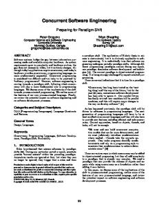
judgment can be used following a bottom-up estimation process. Similarly, it is difficult to distinguish, for example, the Algorithmic and the Top-Down method. Walkerden and Jeffery (Walkerden and Jeffery, 1997) defined a framework consisting of four classes of prediction methods: Empirical, Analogical, Theoretical, and Heuristic. Unfortunately, they state that expert judgment cannot be included in their framework. In addition, the classes Analogy and Heuristic can overlap, as heuristics can be included in the analogy estimation process (see adaptation rules Section 3.5.2). Moreover, it is not evident why methods using Analogy are not empirical as well since certain components of the analogy method can be derived empirically (see similarity functions 3.5.2). Kitchenham (Fenton and Pfleeger, 1996) classifies current approaches to cost estimation into four classes: expert opinion, analogy, decomposition, and models. Here, decomposition can be seen as estimating the effort in a bottom-up manner. Thus, this category overlaps with the other three classes as it not orthogonal to them. Unfortunately, classification schemes are subjective and there is no agreement about the best one (Kitchenham and de Neumann, 1990). Our classification is not fully satisfactory but is designed to follow our argumentation and evaluation regarding the various types of estimation methods. The classification schema is hierarchical, starting from two main categories (Model Based Methods, Non-Model Based Method) that are further refined into sub-categories. The hierarchy should cover all possible types of resource estimation methods, without being overly complicated for our purpose. Such a classification will help us talking in general terms of a certain type of method. Figure 1 summarizes the classification schema we propose for cost estimation methods. The letters in brackets are explained and used in Section 5. Each class is described in the following sub-sections.

Estim ation M ethods

Non-M odel Based M ethods (B)

M odel Based M ethods (A)

G eneric M odel Based (A 1)

Proprietary

Specific M odel Based(A2)

N ot P roprietary D ata D riven

Com posite M ethods

Figure 1: Classification of Resource Estimation Methods

3.1.1

Model Based Methods

Model-based estimation methods, in general, involve at least one modeling method, one model, and one model application method (see Section 5.2). An effort estimation model usually takes a

ISERN 00-05

6

number of inputs (productivity factors and an estimate of system size) and produces an effort point estimate or distribution. •

Generic Model Based These estimation methods generate models that are assumed to be generally applicable across different contexts. • Proprietary: Modeling methods and models are not fully documented or public domain. • Not Proprietary: Modeling methods and models are documented and public domain.

•

Specific Model Based: Specific Model Based estimation methods include local models whose validity is only ensured in the context where they have been developed. • Data Driven: Modeling methods are based on data analysis, i.e., the models are derived from data. We may distinguish here further between parametric and non-parametric modeling methods. Parametric methods require the a priori specification of a functional relationship between project attributes and cost. The modeling method then tries to fit the underlying data in the best way possible using the assumed functional form. Non-Parametric methods derive models that do not make specific assumptions about the functional relationship between project attributes and cost (although, to a certain extent, there are always assumptions being made). • Composite Methods: Models are built based on combining expert opinion and data-driven modeling techniques. The modeling method describes how to apply and combine them in order to build a final estimation model.

3.1.2

Non-Model Based Methods

Non-model based estimation methods consist of one or more estimation techniques together with a specification of how to apply them in a certain context. These methods are not involving any model building but just direct estimation. Usually Non-Model based methods involve consulting one or more experts to derive a subjective effort estimate. The effort for a project can be determined in a bottom-up or top down manner. A top-down approach involves the estimation of the effort for the total project and a splitting it among the various system components and/or activities. Estimating effort in a bottom-up manner involves effort estimates for each activity and/or component separately and the total effort is an aggregation of the individual estimates, possibly involving an additional overhead. 3.2

Description of Selected Methods

There exists a large number of software cost estimation methods. In order to scope down the list of methods we will discuss here, we focus on methods that fulfill the following high-level criteria:

ISERN 00-05

7

1. Recency: We will exclude methods that have been developed more than 15 years ago and were not updated since then. Therefore, we will not discuss in detail models like the WalstonFelix Model (Walston and Felix, 1977), the Bailey-Basili Model (Bailey and Basili, 1981), the SEER (System Evaluation and Estimation Resources) model (Jensen, 1984) or the COPMO (Comparative Programming MOdel) model (Conte et al., 1986). 2. Level of Description: Moreover, the focus is on methods that are not proprietary. We can only describe methods for which the information is publicly available, unambiguous, and somewhat unbiased. Therefore, we will not discuss in detail the generic proprietary methods (“black-box” methods). The level of detail of the description for this kind of methods depends on the level of available, public information. Examples of proprietary estimation methods (and tools) are PRICE-S (Cuelenaere et al., 1987; Freiman and Park, 1979; Price Systems), Knowledge Plan (Software Productivity Research; Jones, 1998), ESTIMACS (Rubin 1985; Kemerer, 1987; Kusters et al., 1990). 3. Level of Experience: We only consider methods for which experience has been gained and reported in software engineering resource estimation. This means an initial utility should already be demonstrated. 4. Interpretability: We will focus on methods for which results are interpretable, i.e., we know which productivity factors have a significant impact and how they relate to resource expenditures. Non-interpretable results are not very likely to be used in practice, as software practitioners usually want to have clear justifications for an estimate they will use for project planning. We will, therefore, not provide a detailed discussion of Artificial Neural Networks. The reader is referred to (Zaruda, 1992; Cheng and Titterinton, 1994).

3.3 3.3.1

Examples of Non-Proprietary Methods COCOMO – COnstructive COst MOdel

COCOMO I is one of the best-known and best-documented software effort estimation methods (Boehm, 1981). It is a set of three modeling levels: Basic, Intermediate, and Detailed. They all include a relationship between system size (in terms of KDSI delivered source instructions) and development effort (in terms of person month). The intermediate and detailed COCOMO estimates are refined by a number of adjustments to the basic equation. COCOMO provides equations for effort and duration, where the effort estimates excludes feasibility and requirements analysis, installation, and maintenance effort. The basic COCOMO takes the following relationship between effort and size

PersonMonth = a( KDSI )b The coefficients a and b depend on COCOMO’s modeling level (basic, intermediate, detailed) and the mode of the project to be estimated (organic, semi-detached, embedded). In all the cases, the value of b is greater than 1, thus suggesting that COCOMO assumes diseconomies of scale. This means that for larger projects the productivity is relatively lower than for smaller projects. The coefficient values were determined by expert opinion. The COCOMO database (63 projects) was used to refine the values provided by the experts, though no systematic, documented process was followed.

ISERN 00-05

8

The mode of a project is one of three possibilities. Organic is used when relatively small software teams are developing within a highly familiar in-house environment. Embedded is used when tight constraints are prevalent in a project. Semi-detached is the mid-point between these two extremes. Intermediate and Detailed COCOMO adjust the basic equation by multiplicative factors. These adjustments should account for the specific project features that make it deviate from the productivity of the average (nominal) project. The adjustments are based on ranking 15 costdrivers. Each cost-driver’s influence is modeled by multipliers that either increase or decrease the nominal effort. The equations for intermediate and detailed COCOMO take the following general form 15

Effort = a Size b ∏ EM i i =1

where EMi is a multiplier for cost-driver i. Intermediate COCOMO is to be used when the major components of the product are identified. This permits effort estimates to be made on a component basis. Detailed COCOMO even uses cost driver multipliers that differ for each development phase. Some adaptations to the original version of COCOMO exist which can cope with adapted code, assess maintenance effort, and account for other development processes than for the traditional waterfall process. In the late 1980’s, the Ada COCOMO model was developed to address the specific needs of Ada projects. The COCOMO II research started in 1994 and is initially described (Boehm et al., 1995). COCOMO II has a tailorable mix of three models, Applications Composition, Early Design, and Post Architecture. The Application Composition stage involves prototyping efforts. The Early Design stage involves a small number of cost drivers, because not enough is known at this stage to support fine-grained cost estimation. The Post Architecture model is typically used after the software architecture is well defined and estimates for the entire development life cycle. It is a detailed extension of the early design model. COCOMO II (Post Architecture) uses 17 effort multipliers and 5 exponential scale factors to adjust for project (replacing the COCOMO I development modes), platform, personnel, and product characteristics. The scale factors determine the dis/economies of scale of the software under development and replace the development modes in COCOMO I. The post architecture model takes the following form. 17

Effort = a Size b ∏ EM i i =1

where b = 1.01 + 0.01

5

ScaleFactor j

j

Major new capabilities of COCOMO II are (1) size measurement is tailorable involving KLOC, Function Points, or Object Points, (2) COCOMO II accounts for reuse and reengineering, (3) exponent-driver approach to model diseconomies of scale, (4) several additions, deletions, and updates to previous cost drivers (Boehm et al., 1996).

ISERN 00-05

9

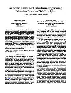
In 1997, a new COCOMO II version included a 10% weighted average approach to adjust the apriori expert-determined model parameters. The underlying database consisted of 83 projects and included 166 data points in 1998. A new version COCOMO II, version 1998, involved Bayesian Statistics to adjust the expert-determined model parameters. Major steps involve to (1) determine a-priori multipliers for cost-drivers using expert judgment (prior information), (2) estimate databased multipliers based on a sample of project data, (3) combine non-sample prior information with data information using Bayesian inference statistics, (4) estimate multipliers for combined information (posterior information). The Bayesian Theorem combines prior information (expert knowledge) with sample information (data model) and derives the posterior information (final estimates) (Chulani et al., 1999). Usually the multiplier information is obtained through distributions. If the variance of an a-priori (expert) probability distribution for a certain multiplier is smaller than the corresponding sample data variance, then the posterior distribution will be closer to the a-priori distribution. We are in the presence of noisy data and more trust should be given then to the prior (expert) information. It is worth noting that COCOMO II is also what we called in Figure 1 a composite method and that we could have described in Section 3.5 too. We decided to leave it in this section as this is also a generic model and this is where the first version of COCOMO is described.

data analysis

Posterior Bayesian update

Prior experts’ knowledge

Figure 2: Example of a prior, posterior, and sample Distribution

Figure 2 illustrates the situation described above and could be the multiplier information for any of the cost-drivers in the COCOMO model. The arrows indicate the mean values of the distributions. In this case, the posterior distribution is closer to the experts’ distribution. 3.3.2

SLIM – Software Life Cycle Management

The Putnam method is based on an equation of staffing profiles for research and development projects (Putnam, 1978), (Londeix, 1987), (Putnam and Myers, 1992). Its major assumption is that the Rayleigh curve can be used to model staff levels on large (>70,000 KDSI) software projects. Plotting the number of people working on a project is a function of time and a project starts with relatively few people. The manpower reaches a peak and falls off and the decrease in manpower during testing is slower than the earlier build up. Putnam assumes that the point in time when the staff level is at its peak should correspond to the project development time. Development effort is assumed to be 40% of the total life cycle cost. Putnam explicitly excludes requirements analysis and feasibility studies from the life cycle.

ISERN 00-05

10

S ta ff L e v e l

T im e

Figure 3: Rayleigh Curve Example

The basic Rayleigh form is characterized through a differential equation

y' = 2 Kat exp ( − at 2 ) y’ is the staff build-up rate, t is the elapsed time from start of design to product replacement, K is the total area under the curve presenting the total life cycle including maintenance, a is a constant that determines the shape of the curve. In order to estimate project effort (K) or development time (td) two equations have been introduced and can be derived after several steps.

[

(

)]

t d = (S ) / D0 C 3 9/7 4/ 7 K = (S / C ) (D0 ) 3

1/ 7

S is system size measured in KDSI, D0 is the manpower acceleration (can take six different discrete values depending on the type of project), C is called the technology factor (different values are represented by varying factors such as hardware constraints, personnel experience, programming experience). To apply the Putnam model it necessary to determine the C, S and D0 parameters up-front. 3.4

Examples of Data Driven Estimation Methods

This section describes a selection of existing data-driven estimation methods. Key characteristics and short examples are provided for each estimation method. 3.4.1

CART - Classification and Regression Trees

Two types of decision trees are distinguished, called classification and regression trees (Breiman et al., 1984; Salford Systems). The intention of classification trees is to generate a prediction for a categorical (nominal, ordinal) variable (Briand et al., 1999c; Koshgoftaar et al., 1999), whereas regression trees generate a prediction along a continuous interval or ratio scale. In the context of software resource estimation, it is therefore natural to use regression trees. Regression trees classify instances (in our case software projects) with respect to a certain variable (in our case productivity). A regression tree is a collection of rules of the form: if (condition 1 and …and condition N) then Z and basically form a stepwise partition of the data set being used. The dependent variable (Z) for a tree may be, for example, effort (Srinivasan and Fisher, 1995) or productivity (Briand et al., 1998; Briand et al., 1999b; Kitchenham, 1998).

ISERN 00-05

11

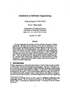
Each node of a tree specifies a condition based on one of the project variables selected. Each branch corresponds to possible values of this variable. Regression trees can deal with variables measured on different scale types. Building a regression tree involves recursively splitting the data set until (binary recursive partitioning) a stopping criterion is satisfied. The key elements to build a regression tree are: (1) recursively splitting each node in a tree in an effective way, (2) deciding when a tree is complete, (3) computing relevant statistics (e.g., quartiles) for each terminal node. There exist several definitions for split criteria. For example, the selection of the variable that maximally reduces the mean squared error of the dependent variable (Salford Systems). Usually splitting generates two partitions but there are other possible approaches (Porter and Selby, 1990). The example in Figure 4 is a regression tree derived from analyzing European Space Agency projects (Briand et al., 1998). Each terminal node represents the average productivity of projects that are characterized by the path from the root. Each node has a condition. If a condition is true then the path on the left is taken. On the first level of the tree, projects are first split according to their team size. If the team size is lower or equal to 7 persons, these projects are split further according to their category. For 29 projects the team size is lower or equal to 7 persons; 27 projects have a team size greater than 7 persons. Following the left branch: Projects falling in the categories “on board systems”, or “simulators” have a mean productivity of 0.35 KLOC/PM (thousands of lines of source code per person-month). Projects with more than 7 team members and where tool usage is between low and nominal have a predicted productivity of 0.09 KLOC/PM. This is the case for 16 projects. Tool ≤ nominal would mean no tool or basic lower CASE tools, and higher than nominal would mean upper CASE, project management and documentation tools used extensively. Projects with a team larger than 7 persons and high-very high usage of tools have a predicted productivity of 0.217 KLOC/PM. This holds for 11 projects of the analyzed projects. TEAM ≤ 7

29 observations

27 observations

TOOL ≤=nominal

CATEGORY = On Board OR Simulators 10 observations

Terminal Node 1 Mean productivity 0.35

19 observations


16 observations


11 observations


Figure 4: Example of a Regression Tree

A new project can be classified by starting at the root node of the tree and selecting a branch based on the project’s specific variable value. One moves down the tree until a terminal node is reached. For each terminal node and based on the projects it contains, the mean, median, and quartile values are computed for productivity. These statistics can be used for benchmarking

ISERN 00-05

12

purposes. One can, for example, determine whether a project’s productivity is significantly below the node mean value. More precisely, one may determine in which quartile of the node distribution the new project lies. If the project lies in the first quartile, then it is significantly lower than expected and the reason why this happened should be investigated. Regression trees may also be used for prediction purposes. Productivity for a node can be predicted by using the mean value of the observations in the node (Briand et al., 1998). This requires building the tree only with information that can be estimated at the beginning of a project. 3.4.2

OSR – Optimized Set Reduction

Optimized Set Reduction (OSR) (Briand et al., 1992; Briand et al., 1993) determines subsets in a historical data set (i.e., training data set) that are “optimal” for the prediction of a given new project to estimate. It combines machine learning principles with robust statistics to derive subsets that provide the best characterizations of the project to be estimated. The generated model consists of a collection of logical expressions (also called rules, patterns) that represent trends in a training data set that are relevant to the estimation at hand. The main motivations behind OSR was to identify robust machine learning algorithm which would better exploit project data sets and still generate easy-to-interpret rule-based models. As mentioned, OSR dynamically builds a different model for each project to be estimated. For each test project, subsets of “similar” projects are extracted in the underlying training set. Like regression trees, this is a stepwise process and, at each step, an independent variable is selected to reduce the subset further and the projects that have the same value (or belong to the same class of values) as the test project are retained. One major difference with regression trees is that the selected variable only has to be a good predictor in the value range relevant to the project to estimate. The (sub)set reduction stops when a termination criterion is met. For example, if the subset consists of less than a number of projects or the difference in dependent variable distribution with the parent (sub)set is not significant. A characteristic of the “optimal” subsets is that they are characterized by a set of conditions that are true for all objects in that subset and they have optimal probability distributions on the range of the dependent variable. This means that they concentrate a large number of projects in a small number of dependent variable categories (if nominal or ordinal) or on a small part of the range (if interval or ratio). A prediction is made based on a terminal subset that optimally characterizes the project to be assessed. It is also conceivable to use several subsets and generate several predictions whose range reflects the uncertainty of the model. An example application of OSR for the COCOMO data set (Boehm, 1981) can be found in (Briand et al., 1992). The example rule below consist of a conjunction of three of the COCOMO cost-drivers (required reliability, virtual machine experience, data base size): RELY=High AND VEXP=High AND DATA=Low => 299 LOC/Person-Month Such logical expression is generated for a given test project and is optimal for that particular project. This project’s productivity can be predicted based on the probability distribution of the optimal subset, e.g., by taking the mean or median. In addition to a point estimate, a standard deviation can easily be estimated based on the subset of past projects characterized by the rule. Because OSR dynamically generates patterns that are specific and optimal for the project to be estimated, it uses the data set at hand in a more efficient way than, say, regression trees.

ISERN 00-05

13

3.4.3

Stepwise ANOVA – Stepwise Analysis of Variance

This procedure combines ANOVA with OLS regression and aims to alleviate problems associated with analyzing unbalanced data sets (Kitchenham, 1998). The values that ordinal and nominal-scale variables can take are called levels. A specific combination of variables and levels is called cells. An unbalanced data set has either unequal numbers of observations in different possible cells or a number of observations in the cells that are disproportional to the numbers in the different levels of each variable. Most software engineering data sets are unbalanced and therefore impacts of variables may be concealed and spurious impacts of variables can be observed (Searl, 1987). The Analysis of Variance (ANOVA) usually decides whether the different levels of an independent variable (e.g., a cost factor) affect the dependent variable (e.g., effort). If they do, the whole variable has a significant impact. ANOVA is used for ordinal or nominal variables. The stepwise procedure applies ANOVA using each independent variable in turn. It identifies the most significant variable and removes its effect by computing the residuals (difference between actual and predicted values). ANOVA is then applied again using the remaining variables on the residuals. This is repeated until all significant variables are identified. Ratio and interval variables can be included in this procedure. Their impact on the independent variable is obtained using OLS regression (for a description of regression see Section 3). The final model is an equation with the most significant factors. For example: if RELY (Reliability) with three levels, and RVOL (Requirements Volatility) with two levels were found to be the most significant, the final model was: Predicted Productivity = µ1,1RELY + µ1,2RELY + µ1,3RELY + µ2,1RVOL + µ2,2RVOL Where, µ, is the mean productivity value in case the cost-driver has the value . In this example, the cost-driver RVOL is identified as significant in the second iteration after the effect of RELY was removed. 3.4.4

OLS – Ordinary Least Squares Regression

Ordinary least-square regression (OLS) assumes a functional form relating one dependent variable (e.g., effort), to one or more independent variables (i.e., cost drivers) (Berry and Feldman, 1985). With least-squares regression, one has first to specify a model (form of relationship between dependent and independent variables). The least squares regression method then fits the data to the specified model trying to minimise the overall sum of squared errors. This is different, for example, from machine learning techniques where no model needs to be specified beforehand. There are several commonly used measures/concepts when applying regression analysis. We will shortly explain their meaning. For further details, refer to (Schroeder et al., 1986). In general, a linear regression equation has the following form2:

DepVar = a + ( b1 × IndepVar1 ) + ... + ( bn × IndepVarn )

2 If the relationship is exponential, the natural logarithm has to be applied on the variables involved and a linear regression equation can be used

ISERN 00-05

14

Where DepVar stands for dependent variable and the IndepVar’s are the independent variables. The dependent variable is the one that is to be estimated. The independent variables are the ones that have an influence on the dependent variable. We wish to estimate the coefficients that minimise the distance between the actual and estimated values of the DepVar. The coefficients b1…bn are called regression coefficients and a is referred to as the intercept. It is the point where the regression plane crosses the y-axis. Four functional forms have been investigated in the literature for modeling the relationship between system size and effort. These are summarized in Table 1 (Briand et al., 1999a).

Model Specification Effort = a + (b × Size) Effort = a + (b × Size) + (c × Size 2 )

Effort = e a × Size b

Effort = e a × Size b × Size c×ln Size

Model Name Linear Model Quadratic Model Log-linear Model Translog Model

Table 1: Functional Forms of Regression-based Effort Estimation Models

The statistical significance is a measure of the likelihood for a result to be “true“, i.e., representative of the population. The p-value is the probability of error that is involved in accepting the observed result as valid. The higher the p-value, the more likely the observed relation between a dependent and an independent variable may be due to chance. More precisely, the p-value for one of the coefficients indicates the probability of finding a value that is different from zero, if the value is zero in the population. If the p-value is high then we have weak evidence that the coefficient value is different from zero. In such a case, the corresponding IndepVar may have no impact on the DepVar. For example, a p-value of 0.05 indicates that there is a 5% probability that the relation between the variables is due to chance. In many cases, a pvalue of 0.05 or 0.01 is chosen as an acceptable error level threshold. Model Specification

Parameter Estimates

p-value Std Error

R2

MMRE

0.72

0.48

ln(Effort) = a + (b × ln(KLOC)) + (c × ln(TEAM)) a

6.23