Review Article Message Passing Based Time Synchronization in

Hindawi Publishing Corporation International Journal of Distributed Sensor Networks Volume 2016, Article ID 1280904, 21 pages http://dx.doi.org/10.1155/2016/1280904

Review Article Message Passing Based Time Synchronization in Wireless Sensor Networks: A Survey Mohammad Ali Sarvghadi1 and Tat-Chee Wan2 1

School of Computer Sciences, Universiti Sains Malaysia (USM), 11800 Penang, Malaysia School of Computer Sciences/National Advanced IPv6 Centre (NAV6), Universiti Sains Malaysia (USM), 11800 Penang, Malaysia

2

Correspondence should be addressed to Mohammad Ali Sarvghadi; mas12 [email protected] Received 14 January 2016; Revised 8 March 2016; Accepted 28 April 2016 Academic Editor: Mario Collotta Copyright © 2016 M. A. Sarvghadi and T.-C. Wan. This is an open access article distributed under the Creative Commons Attribution License, which permits unrestricted use, distribution, and reproduction in any medium, provided the original work is properly cited. Various protocols have been proposed in the area of wireless sensor networks in order to achieve network-wide time synchronization. A large number of proposed protocols in the literature employ a message passing mechanism to make sensor node clocks tick in unison. In this paper, we first classify Message Passing based Time Synchronization (MPTS) protocols and then analyze them based on different metrics. The classification is based on the following three criteria: structure formation of the network affected by the synchronization protocol, frequency of synchronization process (synchronization interval), and synchronization message overhead. Proposed protocols are analyzed and evaluated from different perspectives based on available data. A comparison table of the reviewed protocols is presented according to the evaluation metrics. Finally, some potential methods will be proposed to improve the synchronization process.

1. Introduction Wireless sensor networks (WSNs) are installed everywhere in order to get information about the environment nowadays. Sensor nodes enable many applications in the area of WSN ranging from health (human, animal, or plant), military (battlefield monitoring or target tracking), security, commercial [1] and environmental monitoring (traffic), industrial sensing and diagnostics (supply chains), infrastructure protection (water distribution), and disaster prediction (earthquake) to context-aware computing (intelligent home) [2]. They also form the main parts of the new tech wave of Internet of Things (IoT) which can connect appliances in our lives and allow us to control them remotely by means of sensors and actuators. However, there are some challenges in this area which have become the focus of many researchers. The main problem of the sensors is the power supply. The reason is that in many applications they are not mainly powered and use batteries instead to stay alive. If the battery is depleted, they need to be replaced by another sensor which is not feasible in some places and with certain applications such as battlefields and

disaster monitoring. Therefore, researchers strive to reduce the energy consumption of the sensors as much as possible to prolong the sensors’ lifetime. One way to achieve this important goal is to let the sensors sleep when they are idle and are not sensing the environment. This problem can be easily solved by letting the sensors go into sleep mode when they have no data to send and by adjusting them to wake up once in a while to check if there is any event to sense. However, the situation will be problematic especially when two or more sensors in each other’s transmission range send their sensed data simultaneously. There will certainly be data packets collision, and the intended receiver will be unable to receive the intact information. The collision issue affects both the energy consumption and the bandwidth at the same time as the transmitting data is the most energy consuming action [3–6] and the medium will be occupied without delivering the same information. The main issue to ponder here is the way to adjust and handle the sleep and wake mode of the sensors in the sense that they will know the exact time to sleep and wake up. One way is by making the sensors have the same notion of time or by synchronizing the sensors’ internal timers.

2 The rest of this paper is organized as follows: Section 2 discusses the limitations of the message passing mechanism. In Section 3, the criteria of classification and evaluation metrics are described. Some of the traditional protocols in this area are reviewed in Section 4. Section 5 presents all the multihop MPTS protocols and classifies and evaluates them based on criteria and metrics outlined in Section 3. In Section 5.4 (gradient property of protocols), Section 5.5 (single-hop protocols), and Section 5.6 (protocols with no experiment), some protocols that are not the focus of this work are evaluated. It is to be noted that protocols and directions for further researchers are also presented. The related work and conclusion are presented in Sections 6 and 7, respectively.

2. Time Synchronization Limitations It has to be mentioned that time synchronization involves the setting of the sensor nodes timer’s value in such a way that they will show the same value with reasonable accuracy (the accuracy is application based) at the same moment and all the time. When the sensor nodes are deployed in the sensor field, they start functioning but not parallel in time specifically in multihop scenarios (because they cannot hear the broadcast message from the sink node). It means that they start their timers at different phases. Proposed MPTS protocols try to find this phase’s difference by passing messages to each other and by achieving network-wide synchronization which is known as the offset compensation. However, it does not solve the problem as passing messages causes some difficulties for the synchronization process known as message delay uncertainties. According to [7] message delay is composed of (1) send time, (2) access time, (3) transmission time, (4) propagation time, (5) reception time, and (6) receive time. Send time, access time, and receive time are not deterministic. Propagation delay is negligible as it is less than 1 s for 300 meters [8, 9]. The two remaining tenets can be calculated and are more deterministic. Therefore, it is the nondeterministic parts of the message delay that should be estimated. These uncertainties are usually estimated by the time-stamping mechanism. To keep the network synced, the process of message passing and timestamping should be performed frequently since the oscillator of the sensor nodes which generates the clock ticks drifts away over time from 1 𝜇s to 100 𝜇s per second [10–13]. This frequent synchronization has two main defects. First, it increases energy consumption drastically as the transmitting message has the highest level of energy consumption and second it occupies the channel frequently and does not let the sensors pass their sensed data during the synchronization period. Therefore, the estimation of the oscillator drifts leads to the consumption of less energy and avoids the channel being frequently occupied. An estimation of drift is not as easy as an offset. Drift should be measured over time, and it takes some synchronization intervals. Data points should be recorded and in many cases statistical analysis is performed to estimate the oscillator drift. As a result, it is better to measure and compensate offset and

International Journal of Distributed Sensor Networks drift of the nodes’ internal timer which includes measuring the message’s uncertainties in order to have a good MPTS protocol. The aforementioned problems can be solved using many proposed protocols in many different ways. In this paper, we sought to classify the proposed protocols and evaluate them both quantitatively and qualitatively based on different metrics and available data. The next section defines and describes the classification criteria and evaluation metrics.

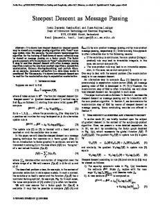
3. Classification Criteria and Evaluation Metrics Existing protocols in this paper are classified based on three criteria: structure [14], synchronization interval, and message overhead. Each of these classes is further expanded into subclasses which are listed and described below. Structure is defined as the way nodes form the network and if there is any specific node(s) that behaves differently from other nodes (root node, cluster head, etc.). A thorough literature inspection shows that existing surveys classify the structure of the network to be centralized and decentralized/distributed [15–17]. However, in this review it is classified as centralized (there is one node known as root or master that starts the synchronization process, and all the other nodes will get synced with the clock of that node), semidistributed (there is more than one node distributed in the network which is responsible for synchronizing the whole network), and fully distributed (all nodes behave in the the same way, and no specific node is included in the network). Synchronization interval refers to how frequent the protocol needs repeat synchronization to keep the network-wide synchronization. It is important for protocols to prolong the synchronization intervals to save more energy [15, 17–19] as multiple messages will be exchanged during each round of synchronization. Therefore, the subclasses of this class are known as short term (those protocols only compensate offset) and long term (those protocols compensate drift as well as an offset). Message overhead relates to how many messages are exchanged between the two nodes in order for one of them (slave) to get synced with the other one (master). Existing surveys normally classify protocols as being 1-way (unilateral) and 2-way (bilateral) [20, 21], but some protocols that exchange 3 messages to get synced are known to exist as well. Therefore, subclasses of this class are one-way (only one message is sent from the master node), two-way (two messages are sent from two nodes consecutively), and threeway (two messages from the master node and one message from slave node are sent). A flowchart of classification is shown in Figure 1. Evaluation metrics for the protocols in this paper are divided into three categories, which are qualitative, quantitative, and other metrics as listed below. It is worth mentioning that, for all evaluation metrics in the tables of this work, firstly, the testbed experiment is considered and if there is no testbed experiment or data, the simulation experiment is considered.

International Journal of Distributed Sensor Networks

3 MPTS

Fully distributed

Semidistributed

1-way 2-way 3-way Hybrid TinySeRSync DMTS PBS TSync CRIT GCS, method 2 DMTS-PBS

Short-term

Long-term

Short-term

1-way

1-way 2-way 3-way

2-way 3-way

RBS ETS

RITS (V1) TDP GCS, method 3 GCS, method 4

ACS Centralized

Short-term

1-way

2-way

GCS, method 1

TPSN LTS

3-way

Long-term

1-way 2-way 3-way RITS (V2) DTSP ATS MTS AOTSP MMTS WMTS

ATSP

Long-term

1-way

2-way

FTSP MH-FTSP RATS LOTS PETSP RSP FBS 2LTSP

SATS BTS TACSC

3-way

Figure 1: MPTS classification chart.

Quantitative metrics are described as follows. (i) Accuracy is one of the key factors of sync protocols [18, 25–28]. The more accurate the protocol, the more the energy saved by sending nodes to sleep mode without any difficulties. In this work, accuracy is defined as the average error between clocks of any two nodes in the whole network (if the average error is not available, the maximum error will be reported). The accuracy is based on clock time and not clock tick as different testbeds or simulation platforms do not have the same crystal oscillator but have different jitters instead. It is to be noted that the accuracy reported in this paper belongs to the maximum hop number. (ii) Energy consumption is the most important factor for WSNs as many application nodes are not mainly powered. Therefore, it is a concern for researchers in this area [21, 26, 29]. Some works attempt to measure energy consumption based on awake and sleep time of the nodes [18] while others try to measure it based on the frequency of message exchange or the number of messages exchanged [28, 30]. In this work, energy consumption is defined as the amount of energy consumed for one round of synchronization to take place in the whole network. However, we do not measure the real energy consumed by one message transmission. However, it is measured by the number of messages exchanged for one cycle of synchronization. Drift is mostly estimated after some

synchronization cycle and when some data points are collected, but in this study, only one cycle is used as energy consumption. (iii) Convergence time is another factor that can consequently affect the protocols and applications that use those protocols [26]. Consider TDMA as an algorithm that uses one of the sync protocols. If the convergence time is too long, it may lead to higher energy consumption as many messages collide and should be resent. If the convergence time is fast enough, it helps protocol to be robust against topology changes and node failure [31]. Convergence time is the duration taken to get network-wide synchronization and is based on clock time and not clock ticks. It is understood that there is no standard threshold for protocols to measure convergence time and each application needs different convergence time based on the accuracy needed for that application. (iv) Experiment topology number of nodes and max hop count are important aspects of experiment. If a protocol can handle a large number of nodes or a large hop count without losing accuracy, it is scalable [25, 26]. (a) Number of nodes is the number of nodes involved in the network. (b) Max hop count is the longest distance between nodes in the network based on the number of hops.

4

International Journal of Distributed Sensor Networks Qualitative metrics are described as follows. (i) Complexity is another concern of researchers [25– 27, 29] as computation load is the second most energy consuming activity that a sensor node can have. Statistical methods normally have high computation load. Therefore, in this survey, if any statistical method or a set of algorithms are used jointly, the protocol is considered complex. (ii) Robustness against node failure describes the behavior of the protocol on node failure [19, 25, 27–29]. In many protocols, there is one or various special node(s) that other nodes get synced with. If any of these nodes fail to service the other nodes, it affects the level of synchronization error at least for a while until another node is replaced by a specific election algorithm. During this time, nodes lose both energy and data. Therefore, any special node in the network is not considered as robust unless the protocol is designed in a way that selecting a new special node(s) does not affect the synchronization process. (iii) Scalability describes the behavior of the protocol if number of hops are increased in the network [19, 27– 29]. In this review, the accuracy of single-hop and multihop scenarios is normally compared. If the level of accuracy decreases linearly or faster than linearly by adding hops, it is considered not scalable. (iv) Synchronization message collision is inevitable before network nodes get synced. MPSPs mostly use CSMA or random waiting time to prevent collision. In both cases, hidden and exposed terminals cannot be promoted. Therefore, if a mechanism is proposed to avoid message collision before getting fully synchronized, the protocol is called collision resistant. Other metrics are described as follows. (i) Proof investigates if the protocol is tested based on a testbed or a simulation platform or theoretically. Protocols tested using testbed experiments are more reliable as simulation experiments are not trustable in many cases [32–34]. (ii) Timestamping investigates if the process is done in Media Access Control (MAC) layer [9]. Therefore, uncertainties of the message delay measurement are minimized to some extent.

The comparisons of the protocols for different metrics are based on available data, and it may not be fair due to different protocol assumptions and different situations or platforms that the protocol is tested through. Protocols are compared and evaluated for the same category. Therefore, at the end of each category, a comparison table is provided based on the evaluation metrics. Section 5 classifies and evaluates the protocols and describes them in their own category. In the context of this survey, the term “message” will mean synchronization message.

Ti−2

B

Ti−1

𝜃

Ti−3

A

Ti

Figure 2: Delay and offset for NTP [22].

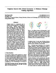
4. Traditional Protocols Before classifying and evaluating MPTS protocols in WSNs, it is worth describing some protocols that form the foundation of many other protocols. Although some protocols are reviewed, none will be classified as they are not included as part of this survey. It is to be noted, however, that the techniques can be used with other protocols too. Some of the protocols do not possess names or short forms for easy addressing or referring. Names have thus been created for each protocol in order to facilitate referring. Network Time Protocol (NTP) [22] is used for different nodes in the Internet. The method used in NTP to get the network-wide synchronization is by calculating the offset through the round trip time (RTT) of the message. The accuracy of 30 ms and 50 ms is the best and worst cases of NTP, respectively. Equation (1) calculates the round trip delay and offset of node B relative to node A at time 𝑇𝑖 . Figure 2 illustrates the scenario. Consider {𝑎 = 𝑇𝑖−2 − 𝑇𝑖−3 { 𝑏 = 𝑇𝑖−1 − 𝑇𝑖 {

{ { RTT = 𝑎 − 𝑏 󳨐⇒ { {offset = (𝑎 + 𝑏) . 2 {

(1)

The later accuracy of NTP [35] is improved to 10 ms for the best case through Phase Lock Loop (PLL) which reduces the phase error of the oscillator. Another NTP [36] is proposed which employs PLL together with Frequency Lock Loop (FLL) and that reduces frequency error as well. This version of NTP [36] improves the accuracy to 1 ms and 100 𝜇s for the worst and best cases, respectively. NTP in general is for the Internet but authors believe it is adequate for wireless networks too. Time Critical Path (TCP) [23] is a revised version of what standard IEEE 802.11 synchronization proposed. Synchronization interval in this protocol is fixed and not based on the order of minutes such as NTP. It achieves the accuracy of 200 𝜇s for an interval of 500 ms. The offset is measured based on sync interval as it is fixed. The precision of the protocol is bounded by Time Critical Pass (the duration that the master node stamps the message and slave node updates its clock). Figure 3 shows the critical path of the TCP protocol. Model Based Protocol (MBP) [24] tries to measure drift as well as offset by collecting a set of three data points of twomessage communication and statistical analysis. It relates the two nodes’ clock by (2) where 𝑎𝑖𝑗 and 𝑏𝑖𝑗 are relative drift and

International Journal of Distributed Sensor Networks

5 T2

Master

B

T3

Slave Time

t1

t2

t3

d

t4 T1

Figure 3: Time Critical Path [23].

A

T4

Figure 5: Offset and propagation delay for TPSN [7]. tji

pj

pi

tij

tij

Figure 4: Two-message mechanism in MBP [24].

offset of two clocks, respectively. Figure 4 presents the twomessage mechanism in MBP. Consider 𝑡𝑖 = 𝑎𝑖𝑗 𝑡𝑗 + 𝑏𝑖𝑗 .

(2)

Post-Facto Synchronization (PFS) [37, 38] starts the synchronization after the occurrence of an event and it removes a huge number of messages exchanged to keep the network synced. However, this kind of protocols is suitable for those applications that do not need periodic synchronization and network nodes to be synced all the time.

5. MPTS Protocols in WSN In this section, all MPTS protocols in WSN are described, classified, and evaluated. Some of their disadvantages are also highlighted to assist researchers to overcome those problems. 5.1. Centralized Protocol 5.1.1. Short-Term Class (1) One-Way Subclass. Global Clock Synchronization (GCS) (method 1: all-node-based) [39] is suitable for a network with small number of nodes. It assumes that drift and processing delay for all nodes are the same and clock tick takes a longer time than transmitting a message. It first finds a loop in all the nodes in the network and then calculates the round trip time of a message along that loop. Nodes pass the message along the loop and update the hop count section of the message. Another message is sent which includes the round trip time and the total number of hops. The nodes adjust their clocks once the message is received. All-Node-Based Limitations. In the case of node failure, the loop should be reformed and this is costly in terms of both energy and time.

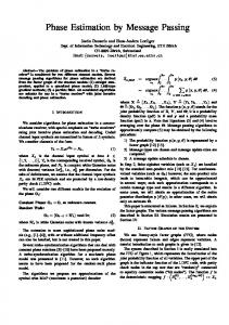
(2) Two-Way Subclass. Timing sync Protocol for Sensor Networks (TPSN) [7] is an NTP-like protocol that can be event driven in a multihop scenario combined with post-facto synchronization. Therefore, there are two solutions in the multihop scenario. The first is based on a hierarchy which involves all nodes in the network and employs overhearing technique (Figure 7). The second is event driven which involves a small part of the nodes in the synchronization process. Once the hierarchy of network nodes is formed, it starts measuring the offset and propagation delay based on (3), which is illustrated in Figure 5. Delay decomposition of TPSN was earlier pointed to in Section 1. It claims that, by timestamping at the MAC layer, the send time, access time, and receive time are removed. TPSN Limitations. In the case of root breakdown, a new root should be selected which wastes both time and energy. It uses acknowledged message to make sure of the existence of the nodes, but it increases the message overhead at the same time. In spite of MAC layer timestamping, the message to be sent will need time to be assembled and it cannot be estimated easily [32]. Consider (𝑇2 − 𝑇1 ) − (𝑇4 − 𝑇3 ) { { {Δ (offset) = 2 { { {𝑑 (delay) = (𝑇2 − 𝑇1 ) + (𝑇4 − 𝑇3 ) { 2

󳨀→ 𝑇2

(3)

= 𝑇1 + Δ + 𝑑. Lightweight Time Synchronization (LTS) [16] aims to sacrifice accuracy to prolong the synchronization interval. The other goal of LTS is to include only a part of network nodes in synchronization process when nodes are spanning the tree to reduce energy consumption. LTS assumes that a transmission range and drift of the nodes are the same. Bounded clock drift and the creation of spanning tree are inspired by [15] and [40], respectively. LTS relates the accuracy of the protocol to the depth of the spanning tree (9.2 × 𝑑 (deepest node) × 𝜎 (variance per hop in units of time)). However, spanning tree is not a different step, and the tree is spanned in each round of synchronization. It decreases the energy consumption by involving only nodes at the edge of each layer. Figure 6 shows the offset measurement process and (4) calculates the offset. LTS has a distributed version, in which nodes are assumed to have some information such as the drift rate, distance to the root node in terms of hops, and desired accuracy. The nodes try to be resynchronized by at

6

International Journal of Distributed Sensor Networks Table 1: Quantitative criteria for centralized protocols.

Protocol

Accuracy

Energy consumption

GCS (method 1) 3Δ (Δ: clock tick) 2𝜖𝑛 TPSN Hierarchy 𝜖𝑛 22.66 𝜇s Event driven 𝜖𝑠 LTS 1.3 ms 2𝜖𝑠 FTSP Multiple ref 3 𝜇s 𝜖𝑛𝑟 Single ref 17.2 𝜇s MH-FTSP 11.7 𝜇s 𝜖𝑛 RATS 2.7 𝜇s No extra message for synchronization (very low) LOTS 152.5 𝜇s 𝜖𝑙𝑠 PETSP Testbed — 𝜖𝑠 Simulation 86 𝜇s RSP Sync period of 30 s 0.88 𝜇s 𝜖(𝑛 − 𝐿) Sync period of 300 s 3.83 𝜇s Setup phase 𝜖(𝑛|𝐸|) FBS Almost 0 Sync phase 𝜖(𝑛 − 𝐿) 2LTSP 1.9 𝜇s 𝜖𝑛 SATS 31.54 ms 2𝜖𝑛 BTS Linear topology 138.62 𝜇s Setup: 𝜖𝑂(𝐸𝑛) Nonlinear topology 196.54 𝜇s Sync: 2𝜖𝑑SH TACSC 22 𝜇s 2𝜖𝑛

Convergence time Number Max hop count of nodes — — — —

6

5

—

500

18

9 min 12 min — — —

60 59 45 60 9

6 11 10 11 8

— 10 s

5 500

4 6

—

5

4

—

3

2

— —

71 6

70 5

—

9 — 1000

8 8 10

—

𝑛: number of nodes in the network; 𝑠: selected nodes included in sync process; 𝐸: number of edges in the graph; 𝜖: energy used to send out one message; 𝑑SH : number of single hop domains; 𝑙: number of messages stored for linear regression; net: short form of network; 𝑟: number of ref broadcasts to estimate drift; 𝐿: lowest level nodes in spanning tree.

T2 = t1 + D + O

Packet 1 T1

B

A Packet 2 T4 = t3 + D − O

T2

Figure 6: Offset in LTS [16].

least the equal rate (𝜏 − 9.2 × 𝑑 × 𝜎). In distributed version, the nonroot nodes that need to be resynchronized send a request to the root node and all the nodes along that way will be synced. However, such arrangements are not considered to be distributed as the nodes will again get synced with the root node. The results in Table 1 belong to the centralized version of LTS. LTS Limitations. In LTS, as a node distances itself from the root node, the error of synchronization increases and it may

violate the scalability of the protocol. The other disadvantage is that protocol is needed in the selection of the nodes at the edge of each level, and it should be applied in each round of synchronization. This results in consuming more energy. Consider 𝑡2 − 𝑡4 = 𝑡1 − 𝑡3 − 𝐷 + 𝐷 + 2𝑑 󳨀→ 𝑑 (4) 1 = × (𝑡2 − 𝑡4 − 𝑡1 − 𝑡3 ) . 2 5.1.2. Long-Term Class (1) One-Way Subclass. Flooding Time Synchronization Protocol (FTSP) [8] aims to get a network-wide synchronization in the order of micro seconds and scalability up to 100 nodes as well as robustness against topology changes. FTSP deals with uncertainties of radio, namely, Interrupt Handling Time, Encoding Time, Decoding Time, and Byte Alignment Time. To remove the effect of the three first uncertainties, it stores multiple timestamps at the receiver and sender side. However, it uses the normalized version upon sending the message.

International Journal of Distributed Sensor Networks Broadcast range

7 eventTime), least square linear regression (LSLR) is used to compensate the offset and drift.

B

RATS Limitations. Reducing the energy consumption by integrating data and sync messages can be assumed to be a plausible idea, but there should be a mechanism to avoid a collision before the network is synced, because in the case of collision both data and energy will be lost and convergence time will be prolonged.

C

A

Ref node

Figure 7: Synchronization using overhearing technique.

It also uses the benefits of both TPSN and RBS, but no spanning tree creation is involved, and the tree is spanned during synchronization. It measures the clock drift based on previous consistent data points through linear regression as it believes that the offset between two nodes is linear. It has two fashions of single reference and multiple references. In order to eliminate redundant messages in multiple reference fashion, FTSP uses some information in both the message and nodes to detect redundant messages. FTSP Limitations. The number of messages exchanged is high and in a dense network the chance of collision is high. Multihop FTSP (MH-FTSP) [41] is another multihop version of FTSP that follows all the rules of a single hop and assumes a connected network during a network lifetime, but in this version, to avoid multiple root election it uses the lowest node ID as the root. MH-FTSP focuses on the robustness against network changes such as a node failure or adding nodes to the network. The experiment shows encouraging results in spite of a highly dynamic network, but when the root node goes down, the percentage of the synchronization reduces from 100% to 55% for a few minutes. MH-FTSP Limitations. We do not classify MH-FTSP as a robust protocol as in some applications, (medical applications) the data is sensitive and losing data for even a few minutes can affect the functionality of the applications. Rapid Time Synchronization (RATS) [42] starts the synchronization from the sink and employs both elapsed time on arrival (ETA) [42] and Routing Integrated Time Synchronization (RITS) [42] (which will be explained in Section 5.3.1(1)), to get network-wide synchronization. Message broadcasted by the sink accommodates two fields which are rootEventTime and eventTime that are initialized to the current time of the sink. rootEventTime is intact during traversing the network while eventTime will be modified based on ETA. After collecting enough data points (rootEventTime and

Low Overhead Time-Sync (LOTS) [43] creates hierarchy by means of messages. A reference node starts broadcasting a message and it continues level by level until all the nodes in the network receive the message. After receiving 𝑚 number of messages, the nodes estimate the offset and drift by linear regression. To discard redundant broadcasts, messages have a sequence number which is increased by the reference node. Therefore, the same messages from different nodes will be discarded. Another technique to prevent message redundancy is through allowing those nodes with specified degree of connectivity with the next level to start broadcasting a message to the upper level. LOTS Limitations. In spite of reducing message redundancy and collision by random waiting time before transmitting, hidden terminal can still lead to collision specifically in dense networks which results in extending the convergence time. This is due to many messages exchanged in one period of synchronization. Another aspect to account for is the fact that finding nodes that have a higher degree of connectivity needs one to maintain a table of neighbors, and more messages should be exchanged to get connectivity info. Message exchange should be done again to find nodes with more connectivity by changing the topology of the network. Power Efficient Timing Synchronization Protocol (PETSP) [44] reduces the energy consumption by decreasing the number of messages exchanged. It adopts the Carrier Sense Multiple Access with Collision Avoidance (CSMA/CA) of 802.11 to access the medium. As it is designed for multihop networks, PETSP selects nodes that cover a larger area to broadcast timing information, and it is to be noted that not all the nodes do synchronization operations. It assigns the node with the lowest ID to be reference node like MH-FTSP [41] and to avoid reference node failure, multiple backup nodes are selected. PETSP strives to teach nonreference nodes to adapt themselves to the speed of reference node’s clock by (5) (𝑡1 , 𝑡2 receiver side and 𝑇𝑆1 , 𝑇𝑆2 sender side). PETSP Limitations. It is robust as no election is required for reference node failure. This is because multiple references are selected, but it is assumed that the preselected reference nodes’ batteries are depleted. Therefore, another election is needed to find the node which covers more nodes in the network, which is both time and energy consuming. Consider 𝑓𝑖 =

𝑡2 − 𝑡1 . (𝑇𝑆2 − 𝑇𝑆1 ) − (𝑡2 − 𝑡1 )

(5)

8

International Journal of Distributed Sensor Networks

Ratio-based time Synchronization Protocol (RSP) [45] is a tree-based structure and all the nodes in the network get synced with the root of the tree. However, the tree is formed during synchronization operation like [8]. The main idea is that the root node sends two messages continuously, and nodes in the broadcast range of the root node receive the two messages and update their clock value according to (6). RSP believes that, due to lack of strong computational resources on the sensor nodes, a short period of resynchronization affects the accuracy because of the numbers after the decimal point. On the other hand, long period of resynchronization affects the accuracy due to clock drift. Therefore, it requires a threshold 𝛼 to update the clock value. If the value of 𝑇3 − 𝑇1 is more than the threshold, it uses previous data point recorded in the memory of the node (in which 𝑇3 − 𝑇2 is more than threshold 𝛽) to apply in (6) (𝑇1 and 𝑇3 are at sender side. 𝑇2 and 𝑇4 are at receiver side. 𝑇𝑠 and 𝑇𝑅 are non-ref nodes and ref nodes, resp.). RSP Limitations. In case of node failure, the nodes should find another parent and this can be costly in terms of both time and energy. The chance of collision is high too as no mechanism is used to minimize message collision. Consider 𝑇𝑅 × 𝑇𝑆

𝑇3 − 𝑇1 (𝑇1 × 𝑇4 ) − (𝑇2 × 𝑇3 ) + . 𝑇4 − 𝑇2 (𝑇4 − 𝑇2 )

(6)

Feedback-Based Synchronization (FBS) [46] aims to employ modified PLL used in SCSP [47]. In FBS, the tree is first constructed, and the synchronization operations are then performed. It tries to ease the effect of internal and external disturbance of the oscillator during the time the node is in sleep mode. FBS Limitations. Since it has a separate setup phase, any changes in the network will force the protocol to accomplish the setup phase again. It does not consider message collision as well. Long-term and Large scale Time Synchronization Protocol (2LTSP) [48] is a protocol in which the intermediate nodes do not change the value of the reference node in sync messages until it reaches the source nodes. In this manner, the synchronization error will not be accumulated in trajectory from the reference node to the source node and leads to the removal of spatial accumulative effect. This means having more hops in the network will not affect the accuracy. In 2LTSP, all nodes sync their logical clock with the hardware clock of the reference node by means of a clock transfer function. It believes that quadratic Taylor expansion is more accurate than a linear one as it has no accumulative errors. It stamps messages three times at both the sender’s and receiver’s side to estimate and compensate clock drift (bounded clock drift is assumed) and offset, and it uses a special message to synchronize the network. 2LTSP assumes that environmental condition does not change during synchronization intervals. 2LTSP Limitations. It uses the message sniffer function of the radio which may not be available in all radios.

(2) Two-Way Subclass. Simple, Accurate Time Synchronization (SATS) [49] is an NTP-like protocol in terms of being hierarchical. It must be stated that hierarchy is formed by each round of synchronization. However, to bind the offset and drift, it employs the technique used in MBP [24]. The difference is that it stamps the message twice at the receiver’s side. It believes that storing many data points affects the complexity and increases the computation load as well as message overhead. Therefore, it uses two algorithms of tiny-sync and mini-sync to decrease the number of data points (only four) which leads to less memory usage as well. SATS piggybacks the synchronization info on the data and acknowledges the message to reduce the message overhead as much as possible. SATS Limitations. One problem of SATS is that it is hierarchical and the chance of accumulating error from the sink to the source is relatively high. Another problem is that all the nodes attend the synchronization process and it will increase the chances of collision too. Broadcast Time Synchronization (BTS) [50] benefits from both TSPN and RBS. It first creates a breadth first spanning tree, and then the root node broadcasts the message and assigns only one of the receivers to communicate with it. The rest of nodes in that broadcast domain overhear the message exchange and estimate drift by least square linear regression after collecting 𝑚 number of data points and offset as well. This process is applied in each single-hop domain of the tree to get a network-wide synchronization. In pairwise operation, BTS employs the technique used in Hierarchy Referencing Time Synchronization Protocol (HRTS) [51], but it uses only one channel and the third message is postponed to the first message of the next sync period, but this does not suggest the existence of a three-way synchronization protocol. BTS Limitations. It is right that BTS reduces the number of three messages used in HRTS [51] to two, but the node has to wait for the next sync period to receive the last data point. Temperature-Assisted Clock Self-Calibration (TACSC) [52] compensates clock drift in a new way. As the clock drift changes over time based on the environment’s temperature, TACSC relates the temperature and frequency of oscillator using a parabolic function before the nodes are deployed in the network. It uses statistical analysis to have an accurate estimation of the offset. TACSC Limitations. It assumes that the delays in both sender’s and receiver’s sides are similar and cannot be guaranteed in real scenarios. It only addresses temperature as environmental factor that affects the node’s clock. In fact, there are some other factors like the oscillator’s age and the fluctuation of voltage level that can make significant roles in the clock drift alteration. As reported in Tables 1 and 2, FBS is the most accurate protocol in the centralized category, but it has two phases and exchanges a considerable number of messages to set up

International Journal of Distributed Sensor Networks

9

Table 2: Qualitative criteria and other metrics for centralized protocols. Protocol GCS (method 1)

Complex

Robust

TPSN

Scalable

Collision resistant

✓

✓

LTS FTSP MH-FTSP RATS

✓ ✓ ✓

✓ ✓ —

LOTS

✓

✓ ✓

PETSP

✓ ✓

RSP

✓

FBS

✓

2LTSP

✓

SATS BTS

✓

✓ ✓

TACSC

✓

✓

the network. It is also scalable and not complex. RATS has the lowest energy consumption and the accuracy is relatively good, based on the MAC layer timestamping. It uses a tested experiment where number of nodes and max hop count are considerable. Convergence time is not reported for many protocols in this category. Among all the protocols in this category, the only robust protocol is PETSP, since it considers multiple backups for the reference node. It is also collision resistant as few of the nodes in the network participate in the synchronization process. In addition to PETSP, TPSN, LOTS, and BTS are also protocols that try to reduce collision. In tables such as Table 1, number of nodes and max hop count are related to the experiment run for that specific protocol. This survey prefers testbed experiment and if it is not available then simulation experiment is reported. For better understanding of some notations please refer to the algorithm. 5.2. Semidistributed Protocol 5.2.1. Short-Term Class (1) One-Way Subclass. Delay Measurement Time Synchronization (DMTS) [53] aims to remove all possible delays in the critical path. Message delay breakdown of DMTS is as follows: sender processing delay, media access delay, transmit delay, radio propagation delay, and receiver processing delay. The first two are eliminated by stamping the message when a clear channel is detected through CSMA. Therefore, the only

✓

Proof Theoretically Testbed Simulation Simulation Testbed Testbed Testbed Testbed Simulation Testbed Simulation Testbed Testbed Simulation Theoretically Testbed Simulation Testbed Simulation Theoretically Testbed Simulation

MAC layer timestamping ✓ ✓ ✓ ✓ ✓ ✓

✓

✓ ✓

✓

delay is the receiver processing delay which is estimated by subtracting two data points on the receiver’s side when the message arrives and when the processing of the message is completed. It uses the hierarchy model but the hierarchy is formed by synchronization protocol. DMTS has an election algorithm to elect a master node which all the other nodes get synced with. DMTS Limitations. In case of a master node breakdown, an election algorithm should be run, and it consumes both time and energy. CSMA algorithm cannot handle hidden and exposed terminals which results in losing messages and leads to the consumption of more energy. GCS (method 2: cluster-based) [39] reduces the message overhead of all-node-based (method 1) protocol [39] by making clusters in the network and by assigning cluster heads for each cluster. Cluster heads are then synced with each other using the the first algorithm. This is followed by synching the cluster member with their cluster head by the first method (we imagine the first method in our evaluation). Cluster-Based Limitations. In addition to the disadvantages of all-node-based limitation (method 1) [39], cluster-based limitation is collision prone and has another overhead which is a clustering algorithm. (2) Two-Way Subclass. Pairwise Broadcast Synchronization (PBS) [54] uses the pairwise operation in [55] to estimate and

10 compensate the offset (linear regression is used) and employs the overhearing technique to reduce energy consumption by decreasing the number of message transmissions. In the overhearing technique, two nodes start the synchronization operation, and those nodes in their transmission range can get synced without the exchange of any messages. Multihop PBS is proposed in [56] which consists of hierarchy forming and pair selection. The pair selection in the multihop version is based on the number of nodes in the common transmission range of pairs, but they should not be on the same level assuming a hierarchy for nodes. Figure 7 shows the overhearing technique. Ref node and node A transmit messages to each other; nodes B and C then listen to the transmitted messages and get synced without sending any messages. PBS Limitations. Multihop version has an extra pairwise operation that violates energy efficiency of single-hop version [57]. Selecting the pairs in the network is costly in terms of both time and energy and makes the protocol vulnerable to node failure. The connectivity of nodes in the network should be checked once in a while by exchanging messages. Distributed Multihop Time Synchronization using PBS (DMTS-PBS) [58] tries to solve the problem of extra pairwise operations by proposing a distributed protocol to select pair nodes. Therefore, it employs a level discovery of TPSN [7], greedy distributed algorithm in [57], and pairwise operation in [55]. After the level discovery, nodes transmit information about their neighbors to the upper-level nodes, decide which pair covers more nodes, and finally start the pairwise operation. DMTS-PBS Limitations. In spite of removing extra pairwise operation, messages needed for level discovery are added. Another element needed is the memory to store the list of neighbors. (3) Three-Way Subclass. Time Synchronization (TSync) [51] gets the benefit of two different algorithms of the HRTS and Individual-based Time Request (ITR) Protocol. HRTS is NTP-like and is used in two fashions of single reference and multireference. In HRTS, nodes get synced with a single reference, but the difference with the NTP is that it uses two different channels to reduce collision. Single reference broadcasts a message on a common channel, and a specific node selected by the reference node replies on a clock channel. Finally, another message is broadcasted with measured offset and delay. Therefore, three messages are transmitted, but the second message is only issued by one node at each level of hierarchy, so it is negligible. In multireference fashion, nodes get synced with the reference node that has a lower level number. ITR is used for nodes that for any reason (collision, channel fading, and so on) could not get synced with the reference node. In ITR, a request is sent by the node to get synced to the reference indirectly (multihop). When all the nodes along this path to the reference node are switched to the clock channel specified in the request, actual sync request is sent using the same method and the reference node sends back the time information to that special node.

International Journal of Distributed Sensor Networks TSync Limitations. It has many specific nodes in the network in HRTS (references and specific nodes selected to involve synchronization) which affects the robustness of the protocol in case of node failure. Using multichannel radios reduces collision drastically (hidden and exposed terminal problems are alleviated). It increases the scalability of the protocol like the algorithm proposed in [59]. In synchronization protocols, it can speed up the convergence time, but multichannel radios are more expensive than single channel radios and the focus of this survey is single channel radios. (4) Hybrid of One-Way, Two-Way, and Three-Way Subclasses. Tiny, Secure, and Resilient time Synchronization (TinySeRSync) [60] is a secured time synchronization protocol, but we only focus on the synchronization part. TinySeSync stamps the message after writing the whole data to the radio buffer and removes all uncertainties on the sender’s side. It has two independent phases of pairwise and global synchronization that are performed every 5 and 10 seconds, respectively. Pairwise phase uses (3) to calculate the offset and keep the offset relative to their neighbors. The flow of synchronization in this protocol is from source to sink. At the time of global synchronization, source node broadcasts the sync message. One hop neighbor nodes are aware of their offset relative to the source node. Therefore, they start to broadcast their local clock as well as an offset relative to the source node. This process continues to acquire a networkwide synchronization. TinySeRSync Limitations. The most important problem is the huge message overhead and the idea that collision is inevitable in dense networks. Chained-Ripple Time Synchronization (CRIT) [61] syncs the network in two phases of horizontal missionary node discovery (chained phase) and vertical sensor node synchronization (ripple phase). Synchronization starts with broadcasting a message by a reference node. Reference node is supposed to have a stronger transmission power than all the other nodes. Based on a transmission power, a missionary node (MN) is selected among the nodes in the transmission range of reference nodes. During the process of MN selection, MN gets synced with a reference node by NTP [35] algorithm with some modifications. The process of this phase synchronization is shown in Figure 8 as well as an offset and propagation estimation in (7). MN selection continues using the selected MN to cover the whole network. Then MNs establish Sensor Groups (SG) with their one-hop neighbors. MNs are assumed to have the location, time, and computing resource information of all the nodes in its SG. Hence, this is the time for normal sensor nodes to get synced with their MNs. This process is accomplished by the Distributed Depth First Search (DDFS) proposed in [62] and all the nodes get synced with BS through this way. CRIT Limitations. In the ripple phase, the synchronization error increases according to the number of nodes even in one broadcast domain based on the use of DDFS. Another fact is

International Journal of Distributed Sensor Networks T2 T3

T6

Sender side (A)

Receiver side (B)

T4 T5

T1

11

Figure 8: Chained-Ripple Time Synchronization.

1

A

B

2

3

C

4

D

ETS Limitations. In ETS, there is no guarantee for a hierarchy of selected nodes to be synced well due to reasons such as hidden or exposed terminal. 5

Figure 9: Multihop RBS [10] (modified).

that CRIT needs enough memory for the nodes to keep track of the nodes in each SG. Consider 𝑜=

(𝑇4 − 𝑇3 ) − (𝑇6 − 𝑇5 ) , 2

(𝑇 − 𝑇3 ) + (𝑇6 − 𝑇5 ) 𝑑= 4 . 2

and only record the time included in the message received from the local reference and when enough data points are stored, they apply a linear regression to estimate the offset and drift. In this method, the communication overhead is reduced which will eventually improve the network’s lifetime too. ETS believes that an accurate estimation of the offset depends on an accurate estimation of the drift.

(7)

5.2.2. Long-Term Class (1) One-Way Subclass. Reference Broadcast Synchronization (RBS) [10] removes the nondeterministic parts of the critical path as shown in Figure 3. In fact, it removes the “sent time” and “access time” at the sender’s side. In RBS, a master node sends a nonstamped message to the slave nodes, and they stamp the message based on their local clock and negotiate with their neighbors to find the best estimation through the least square linear regression. Figure 9 shows the multihop version of RBS. As shown, there are some nodes (A, B, C, and D) which play the role of master nodes for the other nodes. Big circles in Figure 9 illustrate the transmission range of master nodes. Master nodes should be synced first, and only then the message should be sent to the slave nodes. Care should be taken so that if one of the master nodes fails, the remaining nodes in the overlapped areas can assist in the synchronization process.

(2) Three-Way Subclass. Adaptive Clock Synchronization (ACS) [64] employs the technique used in RBS, but only after receiving 𝑛 number of messages, it calculates the slope of the line formed by the data points and returns it back to the sender in addition to a point on that line by a random delay to decrease the chance of collision. Afterwards, the master node creates a message of the receivers’ information and broadcasts it. This way, the receivers have information related to their neighbors. Therefore, the number of messages exchanged is drastically alleviated. ACS Limitations. It is right that ACS reduces the number of messages exchanged, but it loses accuracy at the same time, and there is a trade-off between the number of messages exchanged and accuracy. Another problem is that, in the multihop scenario, a considerable number of the messages are sent, and the chance of collision is high in spite of using random delay. As reported in Tables 3 and 4, ETS is the most accurate protocol and uses MAC layer timestamping. Energy consumption is also the best in this category as not all nodes are involved in the synchronization process. The number of nodes is considerable, but it is based on simulation. ETS also uses statistical analysis to estimate drift which makes it complex. It is scalable due to not losing accuracy by increasing the number of hop counts. Except for TSync, tinySeSync, and ACS, all the protocols in this category are not collision resistant, but most of them are not complex. Half of the protocols in this category employ MAC layer timestamping. In spite of being semidistributed, only TinySeSync protocol is robust in this category. 5.3. Fully Distributed Protocol 5.3.1. Short-Term Class

RBS Limitations. In RBS, a large number of messages are transmitted in each cycle of the synchronization. This results in two different problems, the high energy consumption and the high chance of collision. Efficient Time Synchronization (ETS) [63] is an extension of RBS which increases the accuracy of the RBS and leads the RBS to have a longer sync period. In the multihop scenario, it creates a hierarchy based on some selected nodes synced by other nodes. These selected nodes are called the local reference and their responsibility is to broadcast the message. Unlike the RBS, the other nodes do not exchange any message

(1) One-Way Subclass. Routing Integrated Time Synchronization (RITS) (V1) [42] is a post-facto synchronization that uses specific multiple nodes and routes over multiple hops to convey data to the sink node. Therefore, the sink node receives multiple messages and constructs the event times based on different nodes and then forms an average. RITS employs the ETA [42] in every hop towards the sink node. ETA uses the MAC layer timestamping technique in [8] to remove uncertainties in the message delay. ETA adds the elapsed time from the occurrence of the event to a separate field in the data message (which is very efficient in terms

12

International Journal of Distributed Sensor Networks Table 3: Quantitative criteria for semidistributed protocols.

Protocol

Accuracy

Energy consumption

46 𝜇s

2𝜖𝑛

6Δ (Δ: clock tick)

2𝜖𝑛

29.47 48.48 52.08 𝜇s

𝜖(2𝑛 + 𝑠) 3𝜖𝑛󸀠 3𝜖𝑛

12 𝜇s 640 𝜇s 3.68 𝜇s 1.03 𝜇s Function of messages

3𝜖𝑀 𝜖𝑂(𝑛) 𝜖𝑛𝑟 𝜖𝑠𝑟 𝜖(𝑟 + 𝑛)

DMTS GCS (method 2) TSync HRTS ITR TinySeSync CRIT Chained phase Ripple phase RBS ETS ACS

Convergence time Time of sending and receiving 𝑛 messages —

Number of nodes

Max hop count

3

2

—

—

—

5

3

—

60

8

6 100 9 250 —

5 1 8 5 —

— — — 7 ref broadcasts

𝑠: selected local references; 𝑟: number of ref broadcasts to estimate drift; 𝑛󸀠 : number of nodes in specific branch; 𝑀: number of missionary nodes.

Table 4: Qualitative criteria and other metrics for semidistributed protocols. Protocol DMTS GCS (method 2) TSync HRTS ITR TinySeSync

Complex

Robust

✓

Scalable

Collision resistant

Proof Testbed Theoretically

MAC layer timestamping ✓

✓

✓

Testbed

✓

—

✓

✓

✓ ✓ —

✓

Testbed Theoretically Simulation Testbed Simulation Theoretically

CRIT RBS ETS ACS

✓ ✓ ✓

of energy consumption) and broadcasts it. At the receiver’s side, the event time is reconstructed based on the received elapsed time. Since ETA stores the event time during the time the message is being sent, all uncertainties of the message delay are eliminated or highly reduced. RITS is further studied in [65] where RITS is tested without controlling the reporting nodes. All the nodes that detect the event then report it to the sink through different routes and verify the drastic reduction of accuracy (from 7.86 𝜇s to 1.57 ms). This reduction in accuracy is verified through the drift of different nodes. RITS Limitations. It is only suitable for applications that do not need frequent synchronization. GCS (method 3: rate-based synchronous diffusion) [39] is the third method of GCS in which each node 𝑛𝑖 exchanges clock information with its neighbors (𝑛𝑗 ). In the following, neighbors of 𝑛𝑖 change their clock to 𝑐𝑗 + 𝑟𝑖𝑗 (𝑐𝑖 − 𝑐𝑗 ), where 𝑐𝑖 , 𝑐𝑗 , and 𝑟𝑖𝑗 are clock of 𝑛𝑖 , clock of 𝑛𝑗 , and diffusion rate, respectively. 𝑛𝑖 also changes its clock to 𝑐𝑖 − ∑all 𝑛’s neighbors 𝑟𝑖𝑗 (𝑐𝑖 − 𝑐𝑗 ).

✓

Therefore, the nodes get synced to the average difference of all the nodes’ clocks. Rate-Based Synchronous Diffusion Limitations. This algorithm is collision prone and the rate of collision extends the convergence time. One drawback of this method is that it needs a set of extra operations to be performed by the nodes which are removed in method four in the next section. Uncertainties of message exchange are not considered too. GCS (method 4: asynchronous diffusion) [39] is the fourth method of GCS in which each node 𝑛𝑖 asks its neighbor to read the clocks, compute the reading average, and send back the average to all the neighbors as well as itself. Asynchronous Diffusion Limitations. The number of messages exchanged is high which leads to higher chances of collision, and no mechanism is used to avoid a collision. Uncertainties of message exchange are not considered too. (2) Two-Way Subclass. Time Diffusion synchronization Protocol (TDP) [66] starts by sending out a pulse from the reference

International Journal of Distributed Sensor Networks node. By receiving this pulse, the receivers determine if they can be master nodes (those that other nodes can get synced with). The master nodes then broadcast timing information. Subsequently, the nodes get synced with the master nodes and start to select diffused leaders based on similar criteria to how the master nodes were selected. This process continues until all the nodes are synced. The novelty of TDP is that it employs algorithms that do not allow nodes with low energy and false tick to become master nodes or diffusion leaders by means of Election Reelection Procedure (ERP) algorithm. ERP consists of two subalgorithms of False ticker Isolation Algorithm (FIA) and Load Distribution Algorithm (LDA). After that, selected master nodes remove false ticker nodes between themselves using the Peer Evaluation Procedure (PEP). Time synchronization itself is performed by the Time diffusion Procedure (TP) that consists of Time Adjustment Algorithm (TAA) and Clock Discipline Algorithm (CDA) [36]. In spite of having specific nodes in this protocol, node selection is very dynamic and for each round of synchronization new nodes are selected. TDP Limitations. It consists of many different algorithms that should be run in every round of synchronization, which is costly in terms of time and energy. TDP do not compensate the drift and just select the nodes with a reasonable drift in each round. However, a drift can vary due to environmental reasons or oscillator aging. Therefore, in such situations, the frequency of synchronization goes up and affects the energy consumption. TDP uses a three-way message exchange to select the master or diffused leader nodes, but for the synchronization part, it uses only two-way message exchange. 5.3.2. Long-Term Class (1) One-Way Subclass. RITS (V2) [65] is tested again with both the compensating offset and drift. In this version, a table of transmission and received time is recorded in each node to estimate the relative drift. RITS is highly affected by the size of the table which records the data points. In the first experiment, the table size is large enough to keep all the neighbors’ data points. The accuracy of this experiment is promoted to 2.8 𝜇s. Another experiment is established which limits the table size to only 6 records. In this way, RITS estimates the drift for other nodes without any table. The accuracy for this scenario is 5.3 𝜇s. In RITS (V2), the drift’s compensated scalability is promoted as well as its accuracy. RITS (V2) Limitations. When the number of records is reduced to 6, the synchronization error becomes almost doubled. Therefore, accuracy is highly affected by table size. Average TimeSync (ATS) [67, 68] removes message uncertainties by stamping messages after the first bit, Start of Frame Delimiter (SFD), is sent (it is the feature of hardware used). It assumes that the messages are delivered instantly and no processing and message delay are considered. ATS first measures and compensates the drift and then offsets it to a virtual clock and this process continues to reach a consensus. It is resilient to packet loss, node failure, replacement, or

13 relocation. It assumes a strongly connected graph, but only during times when communication is feasible. Equation (8) estimates and updates the drift in which 𝜂𝑖𝑗+ is the new value of 𝜂𝑖𝑗 and it is proven that over time it will be equal to the drift between nodes 𝑖 and 𝑗 (𝛼𝑖𝑗 = 𝛼𝑗 /𝛼𝑖 ), and 𝜌𝜂 and 𝜌𝑦 are tuning parameters. Details in Table 5 belong to [68]. ATS Limitations. No mechanism for preventing a collision is proposed, and it suffers from 5% to 10% message loss which affects the convergence time since the packet loss causes a significant disturbance to the synchronization process. Consider 𝜂𝑖𝑗+ = 𝜌eta 𝜂𝑖𝑗 + (1 − 𝜌eta )

𝜏𝑗 (𝑇2 ) 𝜏𝑗 (𝑇1 ) 𝜏𝑖 (𝑇2 ) 𝜏𝑖 (𝑇1 )

,

(8)

̃ 𝑖 + (1 − 𝜌V ) 𝜂𝑖𝑗 𝛼 ̃𝑖. ̃ +𝑖 = 𝜌eta 𝛼 𝛼 Maximum Time Synchronization (MTS) [69] aims to converge all the nodes’ clocks to the node which has the largest drift and offset. It assumes that the network simulates a strongly connected graph, with no processing time and no message delay and the age of each link is not less than a fixed time. The main contribution of MTS is fast convergence and compensating drift and offset simultaneously. It is called asynchronous as the synchronization period is slightly different in each node and is based on the drift of the node. Convergence is proved theoretically and convergence time is finite. One advantage of MTS is that it converges faster even when there are movements in the nodes. MTS focuses on convergence time, and when it reaches the threshold (≤10−4 ), it stops syncing. MTS Limitations. It does not consider the message collision and no mechanism is used to control this issue. It is not scalable and as for the 20 nodes, around 100 of sync cycles are needed and for the 60 nodes, they need around 820 sync cycles to converge. Accurate On-demand Time Synchronization Protocol (AOTSP) [70] is a post-facto synchronization protocol. It assumes a special radio which lets access to the radio buffer randomly. Message in AOTSP has two fields of ETA (elapsed time on arrival) and tt (transmission time spent by each node in transmitting the field’s ETA). To find the transformation function, the source, sink, and intermediate nodes store two and four data points, respectively. It measures clock drift using the first-order Taylor expansion and advocates low accumulative error. Taylor expansion has a much better precision compared to linear regression which is ℎ𝜇 (ℎ is the hop distance and 𝜇 is the error in the first hop). This is due to the transformation of the residence time of the event in each intermediate node and this way the accumulative error is not effective. Another achievement of AOTSP is that the number of data points does not affect the accuracy. AOTSP Limitations. It claims a relatively low communication complexity but does not take into account the creation of

14

International Journal of Distributed Sensor Networks Table 5: Quantitative criteria for fully distributed protocols.

Protocol

Accuracy

RITS V1

7.86 𝜇s

GCS (method 3) GCS (method 4) TDP RITS V2 Large record table Limited record table ATS MTS Static net Mobile net

High rate of error High rate of error 100 𝜇s

Energy consumption No extra message for synchronization 𝜖𝑛 𝜖𝑛 PEP: 𝜖𝑟(𝑀 + DL) TP: 2𝜖𝑛

Convergence time

Number of nodes

Max hop count

—

45

10

Function of net nodes Function of net nodes

— —

— —

400 s

200

3

2.8 𝜇s 5.3 𝜇s 305 𝜇s

No extra message for synchronization

—

45

10

𝜖𝑛

10 min

35

10

1 clock tick

𝜖𝑛

30

30

AOTSP

[0.0434, 0.0705] ns

—

100

MMTS WMTS DTSP

97.295 𝜇s 9.15 𝜇s 20 𝜇s 0.5642𝜎 (𝜎: message delay standard deviation)

Setup phase: equal to BFS 𝜖(max hop) 𝜖𝑛 𝜖𝑛 2𝜖𝑛

212 sync cycles 47 sync cycles Not meaningful for post-facto sync 6 sync cycles Longer than MTS Bounded

20 30 40

7 30 9

3𝜖𝐿

15 sync cycles

300

—

ATSP

𝐿: number of links in the network; 𝑀: number of master nodes; 𝑟: number of ref broadcasts to estimate drift; DL: number of diffused leaders.

breadth-first tree before the synchronization process. Reporting an event using neighbor nodes has a high probability of collision too. Maximum Minimum Time Synchronization (MMTS) [71] protocol is the revised version of MTS [69]. It shows that MTS is better than ATS due to very low convergence time. However, as MTS updates the clock values based on drift parameters more than 1 clock tick, the drift compensation is always increasing and will decrease if the minimum consensus is used. To rectify this issue, it uses the average of the maximum and minimum clock values to update the nodes’ clocks. This shows that MMTS calculates both the minimum and maximum consensus and then averages them, which solves the aforementioned problem and reaps the benefit of both protocols. MMTS Limitations. Message collision problem is not considered, and it should be more accurate in terms of synchronization error. Weighted Maximum Time Synchronization (WMTS) [72] is an enhanced version of MTS [69] and considers the normal distribution of the processing delay (variance is on the order of microseconds) of the message in each node. This random delay causes incomplete nodes convergence such as MTS [69] and degrades the synchronization accuracy. Since this work is simulated and a random delay is applied, the chances of increasing the drift are considerable. It uses two variables,

one of which holds the clock reference (the one with the highest drift and offset) and the other one keeps track of the reference clock’s distance in terms of hop number. With the same settings and by applying a random bounded delay, WMTS achieves a better accuracy than MTS [69]. Similar to MTS [69], WMTS shows a faster convergence time for dynamic topologies. WMTS Limitations. It applies a small variance for the random delay, and it can be higher in reality. Collision is not considered. (2) Two-Way Subclass. Distributed Time Synchronization Protocol (DTSP) [73] estimates the transmission delay by collecting 𝑁 number of data points (𝑁 = 10 is the best in terms of memory and accuracy (proven in simulation)) and estimates drift using Recursive Least Squares (RLS) and offset based on the transmission delay, respectively. To reduce the offset and drift between nodes, DTSP applies voltage Kirchhoff law in each loop of the network. In order to remove uncertainties in message transmission, it fills the timestamp field after the first byte is sent. Convergence of DTSP is analyzed in [74]. DTSP Limitations. Finding the different loops in the network is costly in terms of time and energy and in the case of node failure it should be repeatedly done and it affects the robustness of the protocol.

International Journal of Distributed Sensor Networks

15

Table 6: Qualitative criteria and other metrics for fully distributed protocols. Protocol

Complex

Robust

RITS V1 GCS (method 3)

✓

GCS (method 4)

✓

Only for small nets

✓

✓

RITS V2

✓

—

ATS

✓

✓

MTS

✓

TDP

Collision resistant

Scalable

✓

AOTSP MMTS

✓

WMTS

✓

DTSP ATSP

—

✓ ✓

—

(3) Three-Way Subclass. Average Time Synchronization Protocol (ATSP) [75] uses a switching signal to activate the links between a pair of nodes at a time. Then, those pairs start the synchronization operations by estimating offset, drift, and message delay. It continues until all the links in the network are activated. Subsequently, the nodes stop synchronizing until the next period of synchronization. This process carried on until it reaches a consensus. ATSP Limitations. The convergence time of the protocol is long as the synchronization period is extended due to switching signal. As reported in Tables 5 and 6, AOTSP is the most accurate protocol of this category, and the energy consumption is equal to the breadth first search algorithm. Convergence time is not important for AOTSP as it is post-facto. However, it is not complex, robust, or scalable. The result of the test is based on simulation too. ATSP is also accurate, and its accuracy is a function of message delay. Energy consumption is considerable but convergence time is relatively fast. A larger number of nodes are involved in the network, but it is still robust and collision resistant as well as low in complexity. In this category, most of the protocols are robust and are not complex as they are fully distributed. Energy consumption of RITS is the lowest one as it does not use extra message for the synchronization process, but it is only suitable for small networks. 5.4. Gradient Characteristic of Protocols. In this section, the gradient behavior of the protocols is studied. It relates to how the protocols behave as the nodes get distanced from the reference node.

✓

Proof

MAC layer timestamping

Theoretically Theoretically Theoretically Simulation Theoretically Simulation Testbed Theoretically Testbed Theoretically Simulation Theoretically Simulation Theoretically Testbed Theoretically Simulation Testbed Simulation Theoretically Simulation

— — —

✓ ✓ — — ✓ — ✓ —

Gradient Clock Synchronization (1) (GCS(1)) [76] claims that the lower bound of the offset’s worst case for any two nodes in the network is Ω(𝑑 + log 𝐷/ log log 𝐷), where 𝑑 is the distance of the nodes in terms of hop number and 𝐷 is the maximum hop distance in the network. It implies that if the number of nodes in the network increases, the clock offset after performing synchronization increases too. This result is under the assumption that neither link nor node failure is considered and the maximum clock drift and message delay are determined. In addition, clock adaptation time is zero. Meier and Thiele [11] in addition to confirming the lower bound of offset worst case propose a lower bound for gradient drift. However, they assume that communication frequency is bounded by the application as well as assumptions in [76]. They use the main application message to deliver the time information. The proposed lower bound is (𝑑𝜌/8(1 + 𝜌))(log(𝑛 − 1)/ log(8(1 + 𝜌)/𝜌) log(𝑛 − 1)) in which 𝜌 is the upper bound of the clock drift and d is the hop distance of the two nodes. Oblivious Gradient Clock Synchronization (OGCS) [77] proposes the same assumptions as previous algorithms, but it denotes that nodes are unaware of message delay, and that justifies the oblivious label given. OGCS aims to minimize an offset between the neighboring nodes. It proves that many algorithms do not reach the lower bound as proposed in [76]. This matter has been proven in three different versions of algorithms, namely, minimizing the offset to the slowest node, all neighbors (average), and fastest node. Finally, it proposes an algorithm which has the worst case offset of 𝑂(𝑑 + sqrt𝐷) for any two nodes at distance 𝑑. In this algorithm, the nodes not only follow the fastest node’s clock

16 but also consider the slowest node due to clock updating procedure and this method prevents large offset between nodes in the network. Clock Synchronization with Gradient Property (CSwGP) [78] in addition to previous algorithm assumptions assumes that neighbor nodes can communicate in the same direction for a fixed period (embeds timing information of the nodes in data messages and reduces the communication overhead), and the nodes are aware of the diameter of the network and their neighbor’s set. It attempts to adapt the clock drift of a node with the slowest clock rate and the offset with the highest clock value in its vicinity. In previous algorithm [77], there was a controlling component to prevent larger offset between nodes which was a function of the network diameter and there was a lower bound for clock progress in which the nodes were not allowed to evolve below that bound for a fixed period, but in CSwGP the controlling component is constant, and the lower bound is a function of network diameter. This is the reason it reduces the clock offset for the neighboring nodes to the worst case 𝑂(1). Gradient Clock Synchronization Protocol (GTSP) [12] assumes that hardware clock drift is bounded. Unlike previous three algorithms, it considers the link and node failure and uses separate messages to perform synchronization. One benefit of GTSP is to reduce the energy consumption by dynamically changing the synchronization interval (in steady states it is increased which leads to less message exchange). It uses a specific radio which is byte-oriented and stamps sync messages on both sides of the sender and receiver to smooth interrupt jitter. To compensate the clock drift and offset, it considers the average of the nodes’ clock values. Previous studies were based on theoretical aspects, but GTSP is experimentally proven. External Gradient time Synchronization (EGSync) [79] aims to get synchronization as those accomplished in GTSP [12]. However, it uses a node as a reference which can cover the whole network. It aims for nodes to synchronize their offset and drift with reference and neighbor nodes simultaneously. The goal is to develop an algorithm that allows the nodes to get synced with an external clock. For the sake of drift estimation and compensation, it employs linear regression. Two main assumptions of EGSync are bounded drift and bounded message delay of sync message. Gradient Protocols Limitations. Except for the two last protocols, the rest are theoretically analyzed and are unable to reflect the real gradient behavior of the protocols. All protocols are studied under different ideal assumptions that violate reflections of real life scenarios. EGSync is only suitable for application which can accommodate a reference node with a long transmission range that makes the network heterogeneous in terms of the network nodes. If GPS is used, it will only be useful for outdoors applications. As shown in Tables 7 and 8, GTSP is more accurate than EGSync although both use the same energy consumption. Convergence time of GTSP is too long and for EGSync, it is not reported. Both have an acceptable number of nodes for the testbed experiment and are scalable. GTSP employs MAC layer timestamping and is robust, but EGSync is complex.

International Journal of Distributed Sensor Networks Conclusively, GTSP is leading based on the mentioned criteria. 5.5. Single-Hop Protocols. In this section, those protocols with only single-hop scenarios are surveyed. As explained in Section 3, scalability of the protocols is based on the comparison of single-hop and multihop scenarios. Since no multihop is available for these protocols, scalability cannot be evaluated. There will be no classification criteria except for message overhead as we report some centralized and long-term protocols but evaluation metrics are based on the metrics in Section 2 and available data. 5.5.1. One-Way Subclass. Time Synchronization for ZigBee (TSZigBee) [80] is the extension of FTSP [8] which proves coupling FTSP [8] with master-slave star topology of ZigBee results in better accuracy and conserves more energy. It needs to be said that the implementation platform is changed from Mica2 to Telos to get a more accurate timestamping. In TSZigBee, slave nodes do not need to send any sync message or adopt low power mode until the next period of synchronization occurs. The advantage of this protocol is that sync frequency does not have a major effect on accuracy as shown in Table 9. Self-Correcting Time Synchronization (SCTS) [81] tries to teach nodes how to update their clock by only receiving the reference timestamp from the master node. In order to achieve this, it simulates a digital PLL and replaces the Voltage-Controlled Oscillator (VCO) using the local crystal oscillators. This removes the possible noises during timestamping. The precision of this protocol is inversely related to the frequency of resynchronization. It also claims that SCTS reduces memory usage and computational load drastically. SCTS Limitations. Synchronization accuracy is of the order of milliseconds, and it is not suitable for many applications in WSN. 5.5.2. Two-Way Subclass. WiFi for Synchronization (WizSync) [82] is a synchronization protocol which uses WiFi Access Points (APs) availability to get network-wide synchronization. APs broadcast periodic messages (every 102.4 ms) handling the network management. These broadcast messages are used to compensate the drift and offset with a rare message exchange (each 4 hours) as accomplished in [83]. WiZSync is a successful protocol in terms of energy consumption as it reduces the energy consumption drastically. Another benefit of WizSync is that each AP can cover multiple hops of nodes since the broadcast range is much more than sensor nodes. WizSync Limitations. Synchronization accuracy is not high enough for many applications (because of different sources of delay in APs broadcast messages). Moreover, with fading of APs signals, it cannot proceed with the synchronization operation. 5.5.3. Three-Way Subclass. Symmetric Clock Synchronization Protocol (SCSP) [47] claims that statistical analysis used

International Journal of Distributed Sensor Networks

17

Table 7: Quantitative criteria for gradient protocols. Protocol

Accuracy

Energy consumption

Convergence time

GTSP

1 𝜇s

𝜖𝑛

30 min

EGSync Line topology Ring topology

29 𝜇s 14 𝜇s

𝜖𝑛

—

Number of nodes Testbed 20 Simulation 100

Max hop count 9 99

20 20

19 20

Table 8: Qualitative criteria and other metrics for gradient protocols. Protocol

Complex

GTSP EGSync

Robust

Scalable

✓

✓

✓

Collision resistant

✓

Proof Testbed Simulation Testbed Simulation

MAC layer timestamping ✓ —

Table 9: Quantitative criteria for single-hop protocols. Protocol TSZigBee TSync = 2 s & Ttest = 2 min TSync = 30 s & Ttest = 2 min TSync = 30 s & Ttest = 120 min SCTS TSync = 50 s TSync = 25 s WizSync SCSP

Accuracy

Energy consumption

Convergence time

Number of nodes

14.94 𝜇s 24.7 𝜇s 20.43 𝜇s

𝜖𝑛

—

2

𝜖

—

10

Negligible 𝜖(𝑛 + 1)

— —

19 10

1.162 ms 1.126 ms 121 𝜇s 11.32 𝜇s

Table 10: Qualitative criteria and other metrics for single-hop protocols. Protocol TSZigBee SCTS WizSync SCSP

Complex

Robust

Collision resistant ✓ Few messages are exchanged ✓

in [8, 73] for estimating a drift will round the estimated errors. Therefore, it uses an averaging method with a tuning parameter to estimate a drift with better accuracy. The experiment is done with and without measuring the drift. Table 9 shows the results of measuring the drift scenario. SCSP Limitations. It removes the complexity of the protocol by eliminating statistical analysis, but it extrapolates the current timestamp of the reference clock based on previous data points, and it can also affect the precision of the timestamp value. As reported in Tables 9 and 10, SCSP is the most accurate in this category and energy consumption is a function of a number of nodes. It is not complex and robust but collision resistant and employs MAC layer timestamping. WizSync has the least energy consumption, but its accuracy is not

Proof Testbed Testbed Testbed Testbed

MAC layer timestamping ✓ ✓ ✓

acceptable. Based on few messages exchanged between nodes, it is not collision prone. 5.6. Protocols with No Experiment. Fault Tolerant Time Synchronization (FTTS) [84] is an extension of TPSN [7] which considers network failure (node breakdown, movement, or energy depletion) and fault clocks (those clocks are different in drift changes). It has two phases of setup and synchronization like TSPN [7], but in FTTS, each node has a list of parents including a parent and two reference nodes to prevent resetup of the network in case of a parent’s breakdown. At the time of delay and offset measurement, each node calculates the average of delay and offset and then removes the nodes which are out of the average bound from the list. It assumes 𝑛 ≤ 3𝑚 + 1, where 𝑛 is the number of nodes in the network and 𝑚 is the number of nodes with faulty clocks. Another

18 assumption is that the clock of root node does not fluctuate and is an ideal clock. Lightweight Fault Tolerant Time Synchronization (LFTTS) [85] is an extension of FTTS [84] in which a maximum offset is defined. Based on the maximum offset, any node that is out of that maximum range will be discarded from the list. This way, more energy is conserved. The protocol selects the parent based on the lowest ID of the nodes. FTTS and LFTTS Limitations. Message collision is still problematic as they employ CSMA. In a different situation of faulty nodes and network failure, they achieve 1.5 to 2 times better performance in terms of accuracy and synchronized ratio, but the message overhead is about three times worse than TSPN [7] as they need to exchange the sync messages using 3 nodes. Adaptive Multihop Timing Synchronization (AMTS) [86] is another enhanced version of TPSN [7]. Unlike TSPN [7] which only measures and compensates offset, AMTS measures and compensates both the offset and the drift. It also adds an evaluation step to the level discovery and the synchronization steps of TSPN [7] that helps save more energy. In the evaluation step, it decides which mode of synchronization (i.e., Always On (AO) and Sensor Initiated (SI)) to use. In AO mode, the synchronization is done periodically, but in SI mode, synchronization starts only when it is needed. During the level discovery and synchronization steps, it monitors the network and collects information such as network traffic, branches of the spanning tree (B), synchronization period (𝜏), and an average number of hops (ℎ). Based on this information, it increases or decreases the synchronization period to save energy and to switch from AO to SI and vice versa. It reduces the energy consumption in terms of a message exchange as well. AMTS Limitations. As it is a structure-based protocol, it is vulnerable against node failure and topology changes. Root election and level discovery should be done once a change in the network occurs which may lead to higher energy consumption.

International Journal of Distributed Sensor Networks tries to evaluate them using different statistical methods. Among the mentioned related works are MPTS protocols.

7. Discussion and Future Challenges Many synchronization protocols for WSNs which are based on message passing were reviewed in this survey. To improve the robustness of protocols they should be fully distributed; however, as shown in Figure 1, the majority of the reviewed protocols are centralized protocols. In terms of frequency of message passing, protocols should target long-term synchronization to reduce the frequency of synchronization, which is the approach taken by most protocols in the survey. In terms of message overheads, most protocols belong to the one-way synchronization subcategories and, therefore, have lower overheads. Accuracy is another important factor that can play a primary role in the synchronization frequency too. However, many of the protocols have the error of more than 10 𝜇s and it should be improved in future works. More accurate synchronization protocols result in less energy consumption and more accurate time-based application. Proposed protocols in future should improve accuracy without expending excessive amounts of energy (less message passing process). As can be seen in Tables 1, 3, and 5, the convergence time was not reported. However, proving convergence and convergence time are of importance. Many of the protocols have no mechanism to minimize collision before synchronization starts. In many cases, protocols suffer from packet loss which results in more energy consumption and extends the convergence time. If a mechanism which removes or minimizes the collision before the convergence of the nodes can be proposed, it will help the protocols avoid losing 5 to 15 percent of their messages, which leads to better energy savings. As shown in Table 6, most of the fully distributed protocols are robust, but they are not scalable. Scalability should be achieved without drastically degrading accuracy.

Competing Interests The authors declare that they have no competing interests.

6. Related Works A review from 2004 [25] discusses synchronization problems and compares several synchronization techniques. Reference [26] is a more comprehensive review in terms of the selection of criteria for comparison using qualitative and quantitative metrics, which is the approach adopted for this survey. Reference [20] classifies the protocols into four different categories and focuses on signal processing techniques used for measuring and compensating offset, drift, and message delay. Another work which focuses on signal processing methods in addition to message uncertainties is [9]. Reference [9] mentions some advantages and disadvantages of certain main protocols in this era. Reference [29] evaluates more protocols than the aforementioned work and addresses security concerns as well. A work completed in 2011 closely studied signal processing techniques used in protocols and

Acknowledgments This work has been funded by Universiti Sains Malaysia via RUI Grant no. 1001/PKOMP/811336.

References [1] I. F. Akyildiz, W. Su, Y. Sankarasubramaniam, and E. Cayirci, “Wireless sensor networks: a survey,” Computer Networks, vol. 38, no. 4, pp. 393–422, 2002. [2] F. Zhao and L. J. Guibas, Wireless Sensor Networks: An Information Processing Approach, Morgan Kaufmann, Burlington, Mass, USA, 2004. [3] J. L. Hill and D. E. Culler, “Mica: a wireless platform for deeply embedded networks,” IEEE Micro, vol. 22, no. 6, pp. 12–24, 2002.

International Journal of Distributed Sensor Networks [4] G. Anastasi, M. Conti, M. Di Francesco, and A. Passarella, “Energy conservation in wireless sensor networks: a survey,” Ad Hoc Networks, vol. 7, no. 3, pp. 537–568, 2009. [5] B. Bates, A. Keating, and R. Kinicki, “Energy analysis of four wireless sensor network MAC protocols,” in Proceedings of the 6th International Symposium on Wireless and Pervasive Computing (ISWPC ’11), pp. 1–6, IEEE, Hong Kong, February 2011. [6] R. Yan, H. Sun, and Y. Qian, “Energy-aware sensor node design with its application in wireless sensor networks,” IEEE Transactions on Instrumentation and Measurement, vol. 62, no. 5, pp. 1183–1191, 2013. [7] S. Ganeriwal, R. Kumar, and M. B. Srivastava, “Timing-sync protocol for sensor networks,” in Proceedings of the First International Conference on Embedded Networked Sensor Systems (SenSys ’03), pp. 138–149, November 2003. [8] M. Mar´oti, B. Kusy, G. Simon, and A. L´edeczi, “The flooding time synchronization protocol,” in Proceedings of the 2nd international conference on Embedded networked sensor systems (SenSys ’04), pp. 39–49, ACM, 2004. [9] I.-K. Rhee, J. Lee, J. Kim, E. Serpedin, and Y.-C. Wu, “Clock synchronization in wireless sensor networks: an overview,” Sensors, vol. 9, no. 1, pp. 56–85, 2009. [10] J. Elson, L. Girod, and D. Estrin, “Fine-grained network time synchronization using reference broadcasts,” ACM SIGOPS Operating Systems Review, vol. 36, pp. 147–163, 2002. [11] L. Meier and L. Thiele, “Brief announcement: gradient clock synchronization in sensor networks,” in Proceedings of the 24th Annual ACM Symposium on Principles of Distributed Computing (PODC ’05), p. 238, ACM, July 2005. [12] P. Sommer and R. Wattenhofer, “Gradient clock synchronization in wireless sensor networks,” in Proceedings of the International Conference on Information Processing in Sensor Networks, pp. 37–48, IEEE Computer Society, San Francisco, Calif, USA, April 2009. [13] B.-K. Kim, S.-H. Hong, K. Hur, and D.-S. Eom, “Energyefficient and rapid time synchronization for wireless sensor networks,” IEEE Transactions on Consumer Electronics, vol. 56, no. 4, pp. 2258–2266, 2010. [14] M. A. Sarvghadi and T.-C. Wan, “Overview of time synchronization protocols in wireless sensor networks,” in Proceedings of the 2nd International Conference on Electronic Design (ICED ’14), pp. 204–209, Penang, Malaysia, August 2014. [15] E. Anceaume and I. Puaut, “A taxonomy of clock synchronization algorithms,” Publication Interne 1103, 1997. [16] J. van Greunen and J. Rabaey, “Lightweight time synchronization for sensor networks,” in Proceedings of the 2nd ACM International Conference on Wireless Sensor Networks and Applications (WSNA ’03), pp. 11–19, ACM, 2003. [17] I. Bojic and K. Nymoen, “Survey on synchronization mechanisms in machine-to-machine systems,” Engineering Applications of Artificial Intelligence, vol. 45, pp. 361–375, 2015. [18] S. E. Khediri, N. Nasri, M. Samet, A. Wei, and A. Kachouri, “Analysis study of time synchronizationprotocols in wireless sensor networks,” http://arxiv.org/abs/1206.1419. [19] A. R. Swain and R. C. Hansdah, “A model for the classification and survey of clock synchronization protocols in WSNs,” Ad Hoc Networks, vol. 27, pp. 219–241, 2015. [20] B. M. Sadler and A. Swami, “Synchronization in sensor networks: an overview,” in Proceedings of the Military Communications Conference (MILCOM ’06), pp. 1–6, Washington, DC, USA, October 2006.

19 [21] Y.-C. Wu, Q. Chaudhari, and E. Serpedin, “Clock synchronization of wireless sensor networks,” IEEE Signal Processing Magazine, vol. 28, no. 1, pp. 124–138, 2011. [22] D. L. Mills, “Internet time synchronization: the network time protocol,” IEEE Transactions on Communications, vol. 39, no. 10, pp. 1482–1493, 1991. [23] M. Mock, E. Nett, R. Frings, and S. Trikaliotis, “Continuous clock synchronization in wireless real-time applications,” in Proceedings of the 19th IEEE Symposium on Reliable Distributed Systems (SRDS ’00), pp. 125–132, October 2000. [24] M. Lemmon, J. Ganguly, and L. Xia, “Model-based clock synchronization in networks with drifting clocks,” in Proceedings of the Pacific Rim International Symposium on Dependable Computing (2000), pp. 177–184, Los Angeles, CA, USA, 2000. [25] F. Sivrikaya and B. Yener, “Time synchronization in sensor networks: a survey,” IEEE Network, vol. 18, no. 4, pp. 45–50, 2004. [26] B. Sundararaman, U. Buy, and A. D. Kshemkalyani, “Clock synchronization for wireless sensor networks: a survey,” Ad Hoc Networks, vol. 3, no. 3, pp. 281–323, 2005. [27] G. C. Gautam and T. P. Sharma, “A comparative study of time synchronization protocols in wireless sensor networks,” International Journal of Applied Engineering Research, vol. 1, no. 4, p. 691, 2010. [28] B. Kaur and A. Kaur, “A survey of time synchronization protocols for wireless sensor networks,” International Journal of Computer Science and Mobile Computing, vol. 2, no. 9, pp. 100– 106, 2013. [29] P. Ranganathan and K. Nygard, “Time synchronization in wireless sensor networks: a survey,” International Journal of UbiComp, vol. 1, no. 2, pp. 92–102, 2010. [30] D. Djenouri and M. Bagaa, “Synchronization protocols and implementation issues in wireless sensor networks: a review,” IEEE Systems Journal, 2014. [31] R. Gotzhein and T. Kuhn, “Black Burst Synchronization (BBS)—a protocol for deterministic tick and time synchronization in wireless networks,” Computer Networks, vol. 55, no. 13, pp. 3015–3031, 2011. [32] M. A. Sarvghadi and T.-C. Wan, “AN experimental methodology for evaluation of multi-hop medium access control protocols of wireless sensor networks,” in Proceedings of the IEEE International Conference on RFID-Technologies and Applications (RFID-TA ’13), pp. 1–6, Johor Bahru, Malaysia, September 2013. [33] E. Egea-lopez, J. Vales-alonso, A. S. Martinez-sala, P. Pavonmarino, and J. Garc´ıa-HARO, “Simulation tools for wireless sensor networks,” in Proceedings of the International Symposium on Performance Evaluation of Computer and Telecommunication Systems (SPECTS ’05), p. 24, 2005. [34] E. Kolega, V. Vescoukis, and D. Voutos, “Assessment of network simulators for real world WSNs in forest environments,” in Proceedings of the International Conference on Networking, Sensing and Control (ICNSC ’11), pp. 427–432, Delft, Netherlands, April 2011. [35] D. L. Mills, “Precision synchronization of computer network clocks,” ACM SIGCOMM Computer Communication Review, vol. 24, no. 2, pp. 28–43, 1994. [36] D. L. Mills, “Adaptive hybrid clock discipline algorithm for the network time protocol,” IEEE/ACM Transactions on Networking, vol. 6, no. 5, pp. 505–514, 1998. [37] J. Elson and D. Estrin, “Time synchronization for wireless sensor networks,” in Proceedings of the 15th IEEE International

20

[38]

[39]

[40] [41]

[42]

[43]

[44]

[45]

[46]

[47]

[48]

[49]

[50]

[51]

[52]

[53]

International Journal of Distributed Sensor Networks Symposium on Parallel and Distributed Processing (IPDPS ’01), pp. 1965–1970, San Francisco, Calif, USA, 2001. J. Elson and K. R¨omer, “Wireless sensor networks: a new regime for time synchronization,” ACM SIGCOMM Computer Communication Review, vol. 33, no. 1, pp. 149–154, 2003. Q. Li and D. Rus, “Global clock synchronization in sensor networks,” IEEE Transactions on Computers, vol. 55, no. 2, pp. 214–226, 2006. B. Awerbuch, “A new distributed depth-first-search algorithm,” Information Processing Letters, vol. 20, no. 3, pp. 147–150, 1985. M. Maroti, B. Kusy, G. Simon, and A. Ledeczi, “Robust multihop time synchronization in sensor networks,” in Proceedings of the International Conference on Wireless Networks (ICWN ’04), pp. 454–460, June 2004. B. Kusy, P. Dutta, P. Levis, M. Maroti, A. Ledeczi, and D. Culler, “Elapsed time on arrival: a simple and versatile primitive for canonical time synchronisation services,” International Journal of Ad Hoc and Ubiquitous Computing, vol. 1, no. 4, pp. 239–251, 2006. Z. Shang and H. Yu, “A low overhead multi-hop time-sync protocol for wireless sensor networks,” in Proceedings of the IEEE Networking, Sensing and Control (ICNSC ’05), pp. 54–59, March 2005. C.-M. Chao and Y.-C. Chang, “A power-efficient timing synchronization protocol for wireless sensor networks,” Journal of Information Science and Engineering, vol. 23, no. 4, pp. 985–997, 2007. J.-P. Sheu, W.-K. Hu, and J.-C. Lin, “Ratio-based time synchronization protocol in wireless sensor networks,” Telecommunication Systems, vol. 39, no. 1, pp. 25–35, 2008. J. Chen, Q. Yu, Y. Zhang, H.-H. Chen, and Y. Sun, “Feedbackbased clock synchronization in wireless sensor networks: a control theoretic approach,” IEEE Transactions on Vehicular Technology, vol. 59, no. 6, pp. 2963–2973, 2010. P. Sommer and R. Wattenhofer, “Symmetric clock synchronization in sensor networks,” in Proceedings of the 3rd Workshop on Real-World Wireless Sensor Networks (REALWSN ’08), pp. 11–15, ACM, Glasgow, Scotland, April 2008. G. Huang, A. Y. Zomaya, F. C. Delicato, and P. F. Pires, “Long term and large scale time synchronization in wireless sensor networks,” Computer Communications, vol. 37, pp. 77–91, 2014. M. L. Sichitiu and C. Veerarittiphan, “Simple, accurate time synchronization for wireless sensor networks,” in Proceedings of the IEEE Wireless Communications and Networking Conference: the Dawn of Pervasive Communication (WCNC ’03), pp. 1266– 1273, New Orleans, La, USA, March 2003. C. Xu, L. Zhao, Y. Xu, and X. Li, “Broadcast time synchronization algorithm for wireless sensor networks,” in Proceedings of the 1st International Conference on Sensing, Computing and Automation, pp. 2366–2371, Chongqing, China, May 2006. H. Dai and R. Han, “Tsync: a lightweight bidirectional time synchronization service for wireless sensor networks,” ACM SIGMOBILE Mobile Computing and Communications Review, vol. 8, no. 1, pp. 125–139, 2004. Z. Yang, L. He, L. Cai, and J. Pan, “Temperature-assisted clock synchronization and self-calibration for sensor networks,” IEEE Transactions on Wireless Communications, vol. 13, no. 6, pp. 3419–3429, 2014. S. Ping, “Delay measurement time synchronization for wireless sensor networks,” Tech. Rep. IRBTR-03-013, Intel Research Berkeley Lab, 2003.

[54] K.-L. Noh, E. Serpedin, and K. Qaraqe, “A new approach for time synchronization in wireless sensor networks: pairwise broadcast synchronization,” IEEE Transactions on Wireless Communications, vol. 7, no. 9, pp. 3318–3322, 2008. [55] K.-L. Noh, Q. M. Chaudhari, E. Serpedin, and B. W. Suter, “Novel clock phase offset and skew estimation using two-way timing message exchanges for wireless sensor networks,” IEEE Transactions on Communications, vol. 55, no. 4, pp. 766–777, 2007. [56] K.-L. Noh, Y.-C. Wu, K. Qaraqe, and B. W. Suter, “Extension of pairwise broadcast clock synchronization for multicluster sensor networks,” EURASIP Journal on Advances in Signal Processing, vol. 2008, Article ID 286168, 2007. [57] K.-Y. Cheng, K.-S. Lui, Y.-C. Wu, and V. Tam, “A greedy distributed time synchronization algorithm for wireless sensor networks,” in IEEE International Conference on Communications (ICC ’08), pp. 2327–2331, Beijing, China, May 2008. [58] K.-Y. Cheng, K.-S. Lui, Y.-C. Wu, and V. Tam, “A distributed multihop time synchronization protocol for wireless sensor networks using Pairwise Broadcast Synchronization,” IEEE Transactions on Wireless Communications, vol. 8, no. 4, pp. 1764–1772, 2009. [59] E. Toscano and L. Lo Bello, “A multichannel approach to avoid beacon collisions in IEEE 802.15.4 cluster-tree industrial networks,” in Proceedings of the IEEE Conference on Emerging Technologies and Factory Automation (ETFA ’09), pp. 1–9, Mallorca, Spain, September 2009. [60] K. Sun, P. Ning, and C. Wang, “TinySeRSync: secure and resilient time synchronization in wireless sensor networks,” in Proceedings of the 13th ACM Conference on Computer and Communications Security (CCS ’06), pp. 264–277, ACM, Alexandria, VA, USA, November 2006. [61] K.-Y. Shin, K. Y. Lee, and K. Lee, “CRIT: A hierarchical chainedripple time synchronization in wireless sensor networks,” in Proceedings of the IEEE International Conference on Networking, Sensing and Control (ICNSC ’06), pp. 797–802, April 2006. [62] I. Cidon, “Yet another distributed depth-first-search algorithm,” Information Processing Letters, vol. 26, no. 6, pp. 301–305, 1988. [63] B. Wehbi, A. Laouiti, and A. Cavalli, “Efficient time synchronization mechanism for wireless multi hop networks,” in Proceedings of the IEEE 19th International Symposium on Personal, Indoor and Mobile Radio Communications (PIMRC ’08), pp. 1–6, IEEE, Cannes, France, September 2008. [64] S. Palchaudhuri, A. K. Saha, and D. B. Johnson, “Adaptive clock synchronization in sensor networks,” in Proceedings of the 3rd International Symposium on Information Processing in Sensor Networks (IPSN ’04), pp. 340–348, ACM, April 2004. ´ L´edeczi, and P. Dutta, “On the scalability [65] J. Sallai, B. Kus´y, A. of routing integrated time synchronization,” in Wireless Sensor Networks: Third European Workshop, EWSN 2006, Zurich, Switzerland, February 13–15, 2006. Proceedings, vol. 3868 of Lecture Notes in Computer Science, pp. 115–131, Springer, Berlin, Germany, 2006. [66] W. Su and I. Akyildiz, “Time-diffusion synchronization protocol for wireless sensor networks,” IEEE/ACM Transactions on Networking, vol. 13, no. 2, pp. 384–397, 2005. [67] L. Schenato and G. Gamba, “A distributed consensus protocol for clock synchronization in wireless sensor network,” in proceedings of the 46th IEEE Conference on Decision and Control (CDC ’07), pp. 2289–2294, New Orleans, La, USA, December 2007.

International Journal of Distributed Sensor Networks [68] L. Schenato and F. Fiorentin, “Average TimeSynch: a consensusbased protocol for clock synchronization in wireless sensor networks,” Automatica, vol. 47, no. 9, pp. 1878–1886, 2011. [69] J. He, P. Cheng, L. Shi, and J. Chen, “Time synchronization in WSNs: a maximum value based consensus approach,” in Proceedings of the 50th IEEE Conference on Decision and Control and European Control Conference (CDC-ECC ’11), pp. 7882– 7887, Orlando, Fla, USA, December 2011. [70] G. Huang, A. Y. Zomaya, F. C. Delicato, and P. F. Pires, “An accurate on-demand time synchronization protocol for wireless sensor networks,” Journal of Parallel and Distributed Computing, vol. 72, no. 10, pp. 1332–1346, 2012. [71] J. He, H. Li, J. Chen, and P. Cheng, “Study of consensusbased time synchronization in wireless sensor networks,” ISA Transactions, vol. 53, no. 2, pp. 347–357, 2014. [72] J. He, P. Cheng, L. Shi, J. Chen, and Y. Sun, “Time synchronization in WSNs: a maximum-value-based consensus approach,” IEEE Transactions on Automatic Control, vol. 59, no. 3, pp. 660– 675, 2014. [73] R. Solist, V. S. Borkar, and P. R. Kumar, “A new distributed time synchronization protocol for multihop wireless networks,” in Proceedings of the 45th IEEE Conference on Decision and Control (CDC ’06), pp. 2734–2739, San Diego, Calif, USA, December 2006. [74] A. Giridhar and P. R. Kumar, “Distributed clock synchronization over wireless networks: algorithms and analysis,” in Proceedings of the 45th IEEE Conference on Decision and Control (CDC ’06), pp. 4915–4920, December 2006. [75] J. Wu, L. Jiao, and R. Ding, “Average time synchronization in wireless sensor networks by pairwise messages,” Computer Communications, vol. 35, no. 2, pp. 221–233, 2012. [76] R. Fan and N. Lynch, “Gradient clock synchronization,” in Proceedings of the 23rd Annual ACM Symposium on Principles of Distributed Computing, pp. 320–327, ACM, July 2004. [77] T. Locher and R. Wattenhofer, “Oblivious gradient clock synchronization,” in Distributed Computing, pp. 520–533, Springer, 2006. [78] R. M. Pussente and V. C. Barbosa, “An algorithm for clock synchronization with the gradient property in sensor networks,” Journal of Parallel and Distributed Computing, vol. 69, no. 3, pp. 261–265, 2009. [79] K. S. Yildirim and A. Kantarci, “External gradient time synchronization in wireless sensor networks,” IEEE Transactions on Parallel and Distributed Systems, vol. 25, no. 3, pp. 633–641, 2014. [80] D. Cox, E. Jovanov, and A. Milenkovic, “Time synchronization for ZigBee networks,” in Proceedings of the 37th Southeastern Symposium on System Theory (SSST ’05), pp. 135–138, March 2004. [81] F. Ren, C. Lin, and F. Liu, “Self-correcting time synchronization using reference broadcast in wireless sensor network,” IEEE Wireless Communications, vol. 15, no. 4, pp. 79–85, 2008. [82] T. Hao, R. Zhou, G. Xing, M. W. Mutka, and J. Chen, “WizSync: exploiting Wi-Fi infrastructure for clock synchronization in wireless sensor networks,” IEEE Transactions on Mobile Computing, vol. 13, no. 6, pp. 1379–1392, 2014. [83] A. Rowe, V. Gupta, and R. R. Rajkumar, “Low-power clock synchronization using electromagnetic energy radiating from AC power lines,” in Proceedings of the 7th ACM Conference on Embedded Networked Sensor Systems (SenSys ’09), pp. 211–224, ACM, Berkeley, Calif, USA, November 2009.

21 [84] S. Hwang and Y. Baek, “Fault tolerant time synchronization for wireless sensor networks,” in Architecture of Computing SystemsARCS 2006, pp. 480–493, Springer, Berlin, Germany, 2006. [85] S. Hwang, G.-J. Jin, and B. Kim, “Lightweight fault tolerant time synchronization in wireless sensor networks,” in Proceedings of the 5th International Conference on Networked Sensing Systems (INSS ’08), pp. 131–134, Kanazawa, Japan, June 2008. [86] K.-L. Noh and E. Serpedin, “Adaptive multi-hop timing synchronization for wireless sensor networks,” in Proceedings of the 9th International Symposium on Signal Processing and Its Applications (ISSPA ’07), pp. 1–6, IEEE, February 2007.

International Journal of

Rotating Machinery

Engineering Journal of

Hindawi Publishing Corporation http://www.hindawi.com

Volume 2014

The Scientific World Journal Hindawi Publishing Corporation http://www.hindawi.com

Volume 2014

International Journal of

Distributed Sensor Networks

Journal of

Sensors Hindawi Publishing Corporation http://www.hindawi.com

Volume 2014

Hindawi Publishing Corporation http://www.hindawi.com

Volume 2014

Hindawi Publishing Corporation http://www.hindawi.com

Volume 2014

Journal of

Control Science and Engineering

Advances in

Civil Engineering Hindawi Publishing Corporation http://www.hindawi.com

Hindawi Publishing Corporation http://www.hindawi.com

Volume 2014

Volume 2014

Submit your manuscripts at http://www.hindawi.com Journal of

Journal of

Electrical and Computer Engineering

Robotics Hindawi Publishing Corporation http://www.hindawi.com

Hindawi Publishing Corporation http://www.hindawi.com

Volume 2014

Volume 2014

VLSI Design Advances in OptoElectronics

International Journal of

Navigation and Observation Hindawi Publishing Corporation http://www.hindawi.com

Volume 2014

Hindawi Publishing Corporation http://www.hindawi.com

Hindawi Publishing Corporation http://www.hindawi.com

Chemical Engineering Hindawi Publishing Corporation http://www.hindawi.com

Volume 2014

Volume 2014

Active and Passive Electronic Components

Antennas and Propagation Hindawi Publishing Corporation http://www.hindawi.com

Aerospace Engineering

Hindawi Publishing Corporation http://www.hindawi.com

Volume 2014

Hindawi Publishing Corporation http://www.hindawi.com

Volume 2014

Volume 2014

International Journal of

International Journal of

International Journal of

Modelling & Simulation in Engineering

Volume 2014

Hindawi Publishing Corporation http://www.hindawi.com

Volume 2014

Shock and Vibration Hindawi Publishing Corporation http://www.hindawi.com

Volume 2014

Advances in

Acoustics and Vibration Hindawi Publishing Corporation http://www.hindawi.com

Volume 2014