Revisiting Unsupervised Learning for Defect Prediction - arXiv

Revisiting Unsupervised Learning for Defect Prediction Wei Fu, Tim Menzies Computer Science Department, North Carolina State University 890 Oval Drive Raleigh, North Carolina 27606 [email protected],[email protected]

arXiv:1703.00132v1 [cs.SE] 1 Mar 2017

ABSTRACT Collecting quality data from software projects can be time-consuming and expensive. Hence, some researchers explore “unsupervised” approaches to quality prediction that does not require labelled data. An alternate technique is to use “supervised” approaches that learn models from project data labelled with, say, “defective” or “notdefective”. Most researchers use these supervised models since, it is argued, they can exploit more knowledge of the projects. At FSE’16, Yang et al. reported startling results where unsupervised defect predictors outperformed supervised predictors for effort-aware just-in-time defect prediction. If confirmed, these results would lead to a dramatic simplification of a seemingly complex task (data mining) that is widely explored in the SE literature. This paper repeats and refutes those results as follows. (1) There is much variability in the efficacy of the Yang et al. models so even with their approach, some supervised data is required to prune weaker models. (2) Their findings were grouped across N projects. When we repeat their analysis on a project-by-project basis, supervised predictors are seen to work better. Even though this paper rejects the specific conclusions of Yang et al., we still endorse their general goal. In our our experiments, supervised predictors did not perform outstandingly better than unsupervised ones. Hence, they may indeed be some combination of unsupervised learners to achieve comparable performance to supervised. We therefore encourage others to work in this promising area.

KEYWORDS Data analytics for software engineering, software repository mining, empirical studies, defect prediction ACM Reference format: Wei Fu, Tim Menzies. 2017. Revisiting Unsupervised Learning for Defect Prediction. In Proceedings of ACM SIGSOFT SYMPOSIUM ON THE FOUNDATIONS OF SOFTWARE ENGINEERING, PADERBORN, GERMANY, September 2017 (FSE’2017), 11 pages. DOI: 10.1145/nnnnnnn.nnnnnnn

1

INTRODUCTION

This paper repeats and refutes recent results from Yang et al. [48] published at FSE’16. The task explored by Yang et al. was effort-ware Permission to make digital or hard copies of part or all of this work for personal or classroom use is granted without fee provided that copies are not made or distributed for profit or commercial advantage and that copies bear this notice and the full citation on the first page. Copyrights for third-party components of this work must be honored. For all other uses, contact the owner/author(s). FSE’2017, PADERBORN, GERMANY © 2017 Copyright held by the owner/author(s). 978-x-xxxx-xxxx-x/YY/MM. . . $15.00 DOI: 10.1145/nnnnnnn.nnnnnnn

just-in-time (JIT) software defect predictors built from data miners which study software change metrics. They report an unsupervised software quality prediction method that achieved better results than standard supervised methods. We repeated their study since, if their results were confirmed, that this would imply that decades of research into defect prediction [6, 8, 11, 14–16, 18, 22, 23, 25, 26, 30, 35, 36, 38, 46, 48] had needlessly complicated an inherently simple task. The standard method for software defect prediction is learning from labelled data. In this approach, the historical log of known defects is learned by a data miner. Note that this approach requires waiting until a historical log of defects is available; i.e. until after the code has been used for a while. Another approach, explored by Yang et al., uses general background knowledge to sort the code, then inspect the code in that sorted order. In their study, they assumed that more defects can be found faster by first looking over all the “smaller” modules (an idea initially proposed by Koru et al. [24]). After exploring various methods of defining “smaller”, they report their approach finds more defects, sooner, than supervised methods. These results are highly remarkable: • This approach does not require access to labelled data; i.e. it can be applied just as soon as the code is written. • It is extremely simple: no data pre-processing, no data mining, just simple sorting. Because of the remakrable nature of thse results, this paper takes a second look at the Yang et al. results. We ask three questions: RQ1: Do all unsupervised predictors perform better than supervised predictors? Our results show that, when projects are explored separately, the majority of the models learned by Yang et al. perform worse than supervised learners. Results of RQ1 suggest that after building multiple models using unsupervised methods, it is required to prune the worst models. To test that speculation, we built a new learner, OneWay, that uses supervised training data to remove all but one of the Yang et al. models. Using this learner, we asked: RQ2: Is it beneficial to use supervised data to prune away most of the Yang et al. models? Our results showed that OneWay nearly always outperforms the unsupervised models found by Yang et al. The success of OneWay leads to one last question: RQ3: Does OneWay perform better than more complex standard supervised learners? Such standard supervised learners include Random Forests, Linear Regression, J48 and IBk (these learners were selected based on prior results by [11, 18, 26, 30]). We find that in terms of Recall and Popt (the metric preferred by Yang et al.), OneWay performed

FSE’2017, September 2017, PADERBORN, GERMANY better than standard supervised learners. Yet measured in terms of Precision, there was no advantage to OneWay. From the above, we make an opposite conclusion to Yang et al.; i.e., there are clear advantages to using supervised predictors over unsupervised ones. We explain the difference between our results and their results as follows: • Yang et al. reported averaged results across all projects; • We offer a more detailed analysis on a project-by-project basis. The rest of this paper is organized as follows. Section 2 is a commentary on Yang et al. study. Section 3 describes the background and related work on defect prediction. Section 4 explains the effort-ware JIT defect prediction methods investigated in this study. Section 5 describes the experimental settings of our study, including research questions that motivate our study, data sets and experimental design. Section 6 presents the results. Section 7 discusses the threats to the validity of our study. Section 8 presents the conclusion and future work. Note one terminological convention: in the following, we treat “predictors” and “learners” as synonyms.

2

WHAT YANG ET AL. GOT RIGHT

While this paper disagrees the conclusions of Yang et al., it is important to stress that their paper is an excellent example of good science that should be emulated in future work. Firstly, they tried something new. There are many papers in the SE literature about defect prediction. Compared to most of those, the Yang et al. paper is bold and stunningly original. Secondly, they made all their work freely available. Using the “R” code they placed online, we could reproduce their result, including all their graphical output, in a matter of days. Further, using that code as a starting point, we could rapidly conduct the extensive experimentation that leads to this paper. This is an excellent example of the value of open science. Thirdly, while we assert their answers were wrong, the question they asked is important and should be treated as an open and urgent issue by the software analytics community. In our experiments, supervised predictors performed better than unsupervised– but not outstandingly better than unsupervised. Hence, they may indeed be some combination of unsupervised learners to achieve comparable performance to supervised. Therefore, even though we reject the specific conclusions of Yang et al., we still endorse the question they asked strongly and encourage others to work in this area.

3 BACKGROUND AND RELATED WORK 3.1 Defect Prediction As soon as people started programming, it became apparent that programming was an inherently buggy process. As recalled by Maurice Wilkes [47], speaking of his programming experiences from the early 1950s: “It was on one of my journeys between the EDSAC room and the punching equipment that ‘hesitating at the angles of stairs’ the realization came over me with full force that a good part of the remainder of my life was going to be spent in finding errors in my own programs.” It took decades to gather the experience required to quantify the size/defect relationship. In 1971, Fumio Akiyama [1] described

Wei Fu, Tim Menzies the first known “size” law, saying the number of defects D was a function of the number of LOC where D = 4.86 + 0.018 ∗ LOC. In 1976, Thomas McCabe argued that the number of LOC was less important than the complexity of that code [28]. He argued that code is more likely to be defective when his “cyclomatic complexity” measure was over 10. Later work used data miners to propose defect predictors that proposed thresholds on multiple measures [30]. Subsequent research showed that software bugs are not distributed evenly across a system. Rather, they seem to clump in small corners of the code. For example, Hamill et al. [13] report studies with (a) the GNU C++ compiler where half of the files were never implicated in issue reports while 10% of the files were mentioned in half of the issues. Also, Ostrand et al. [39] studied (b) AT&T data and reported that 80% of the bugs like in 20% of the files. Similar “80-20” results have been observed in (c) NASA systems [13] as well as (d) open-source software [24] and (e) softwre from Turkey [32]. Given this skewed distribution of bugs, a cost-effective quality assurance approach is to sample across a software system, then focus on regions reporting some bugs. Software defect predictors built from data miners are one way to implement such a sampling policy. While their conclusions are never 100% correct, they can be used to suggest where to focus more expensive methods such as elaborate manual review of source code [44]; symbolic execution checking [41], etc. For example, Misirli et al. [32] report studies where the guidance offered by defect predictors: • Reduced the effort required for software inspections in some Turkish software companies by 72%; • While, at the same time, still being able to find the 25% of the files that contain 88% of the defects. Not only do static code defect predictors perform well compared to manual methods, they also are competitive with certain automatic methods. A recent study at ICSE’14, Rahman et al. [42] compared (a) static code analysis tools FindBugs, Jlint, and Pmd and (b) static code defect predictors (which they called “statistical defect prediction”) built using logistic regression. They found no significant differences in the cost-effectiveness of these approaches. Given this equivalence, it is significant to note that static code defect prediction can be quickly adapted to new languages by building lightweight parsers that find extract static code metrics. The same is not true for static code analyzers– these need extensive modification before they can be used on new languages. To build such defect predictors, we measure the complexity of software project using McCabe metrics, Halstead’s effort metrics and CK object-oriented code mertics [4, 12, 17, 28] at a coarse granularity, like file or package level. With the collected data instances along with the corresponding labels (defective or non-defective), we can build defect prediction models using supervised learners such as Decision Tree, Random Forests, SVM, Naive Bayes and Logistic Regression [11, 19–21, 26, 30]. After that, such trained defect predictor can be applied to predict the defects of future projects.

3.2

Just-In-Time Defect Prediction

Traditional defect prediction has some drawbacks such as prediction at a coarse granularity and started at very late stage of software development circle [18], whereas in JIT defect prediction paradigm,

Revisiting Unsupervised Learning for Defect Prediction the defect predictors are built on code change level, which could easily help developers narrow down the code for inspection and JIT defect prediction could be conducted right before developers commit the current change. JIT defect prediction becomes more practical method for practitioners to carry out. Mockus et al. [33] conducted the first study to predict software failures on a telecommunication software project, 5ESS, by using logistic regression on data sets consisted of change metrics of the project. Kim et al. [22] further evaluated the effectiveness of change metrics on open source projects. In their study, they proposed to apply support vector machine to build a defect predictor based on software change metrics, where on average achieved 78% accuracy and 60% recall. Since training data might not be available when building the defect predictor, Fukushima et al. [7] introduced crossproject paradigm into JIT defect prediction. Their results showed that using data from other projects to build JIT defect predictor is feasible. Most of the research into defect prediction does not consider the effort1 required to inspect the code predicted to be defective. Exceptions to this rule include the work of Arishom and Briand [2], Koru et al. [24] and Kamei et al. [18]. Kamei et al. [18] conducted a large-scale study on the effectiveness of JIT defect prediction, where they claimed that using 20% of efforts required to inspect all changes, their modified linear regression model (EALR) could detect 35% defect-introducing changes. Inspired by Menzies et al.’s ManualUp model (i.e., small size of modules inspected first) [31], Yang et al. [48] proposed to build 12 unsupervised learners by sorting the reciprocal values of 12 different change metrics on each testing data set in descending order. They reported that with 20% efforts, many unsupervised learners perform better than state-ofthe-art supervised learners.

4 METHOD 4.1 Unsupervised Learner In this section, we describe the effort-aware just-in-time unsupervised defect learner proposed by Yang et al. [48], which serves as a baseline method in this study. As described by Yang et al. [48], their simple unsupervised defect learner is built on change metrics as shown in Table 1. These 14 different change metrics can be divided into 5 dimensions [18]: • • • • •

Diffusion: NS, ND, NF and Entropy. Size: LA, LD and LT. Purpose: FIX. History: NDEV, AGE and NUC. Experience: EXP, REXP and SEXP.

The diffusion dimension characterizes how a change is distributed at different levels of granularity. As discussed by Kamei et al. [18], a highly distributed change is harder to keep track and more likely to introduce defects. The size dimension characterizes the size of a change and it is believed that the software size is related to defect proneness [24, 36]. Yin et al. [49] report that the bug-fixing process can also introduce new bugs. Therefore, the Fix metric could be used as a defect evaluation metric. The History dimension includes some 1 Effort

means time/labor required to inspect total number of files/codes that are predicted as defective

FSE’2017, September 2017, PADERBORN, GERMANY historical information about the change, which has been proven to be a good defect indicator [27]. For example, Matsumoto et al. [27] find that the files previously touched by many developers are likely to contain more defects. The Experience dimension describes the experience of software programmers for the current change because Mockus et al. [33] show that more experienced developers are less likely to introduce a defect. More details about these metrics can be found in Kamei et al’s study [18]. Table 1: Change metrics used in our data sets. Metric NS ND NF Entropy LA LD LT FIX NDEV AGE NUC EXP REXP SEXP

Description Number of modified subsystems [33]. Number of modified directories [33]. Number of modified files [37]. Distribution of the modified code across each file [5, 14]. Lines of code added [36]. Lines of code deleted [36]. Lines of code in a file before the current change [24]. Whether or not the change is a defect fix [9, 49]. Number of developers that changed the modified files [27]. The average time interval between the last and the current change [8]. The number of unique changes to the modified files [5, 14]. The developer experience in terms of number of changes [33]. Recent developer experience [33]. Developer experience on a subsystem [33].

In Yang et al.’s study, for each change metric M, they build an unsupervised learner that ranks all the changes based on the corresponding value of M1(c) in descending order, where M(c) is the value of the selected change metric for each change c. Therefore, the changes with smaller change metric values will ranked higher. In all, for each project, Yang et al. define 12 simple unsupervised learners (LA and LD are excluded as Yang et al. [48]).

4.2

Supervised Learner

To further evaluate the unsupervised learner, we selected some supervised learners that already used in Yang et al.’s work. As reported in both Yang et al.’s [48] and Kamei et al.’s [18] work, EALR outperforms all other supervised learners for effortaware JIT defect prediction. EALR is a modified linear regression Y (x) model [18] and it predicts Effort(x) instead of predicting Y (x), where Y (x) indicates whether this change is a defect or not (1 or 0) and Effort(x) represents the effort required to inspect this change. Note that this is the same method to build EALR as Kamei et al. [18]. In defect prediction literature, IBk (KNN), J48 and Random Forests methods are simple yet widely used as defect learners and have been proven to perform, if not best, quite well for defect prediction [11, 26, 30, 45]. These three learners are also used in Yang et al’s study. For these supervised learners, Y (x) was used as the dependant variable. For KNN method, we set K = 8 according to Yang et al. [48].

4.3

OneWay Learner

Based on our preliminary experiment results shown in the following section, for the six projects investigated by Yang et al, some of 12 unsupervised learners do perform worse than supervised learners.

FSE’2017, September 2017, PADERBORN, GERMANY This means we can not say which simple unsupervised learner works for the new project before testing. In this case, we need to select the proper metric to build unsupervised learners. We propose OneWay learner, which is supervised learner built on the idea of simple unsupervised learner. The pseudocode for OneWay is shown in Algorithm 1. In the following description, we use the superscript numbers to denote the line number of pseudocode. Algorithm 1 Pseudocode for OneWay Input: data train, data test, eval goal ∈ {F1, Popt , Recall, Precision, ... } Output: result 1: 2: 3: 4: 5: 6: 7: 8: 9: 10: 11: 12: 13: 14: 15: 16: 17: 18: 19: 20: 21: 22:

function OneWay(data train, data test, eval goal) all scores ← NULL for metric in data train do learner ← buildUnsupervisedLearner(data train, metric) scores ←evaluate(learner) //scores include all evaluation goals, e.g., Popt, ACC, ... all scores.append(scores) end for best metric ← pruneFeature(all scores, eval goal) result ← buildUnsupervisedLearner(data test, best metric) return result end function function pruneFeature(all scores, eval goal) if eval goal == NULL then mean scores ← getMeanScoresForEachMetric(all scores) best metric ← getMetric(max(mean scores)) return best metric else best metric ← getMetric(max(all scores[“eval goal”])) return best metric end if end function

The general idea of OneWay is to use supervised training data to remove all but one of the Yang et al. models. Specifically, OneWay firstly builds simple unsupervised learners for each metric on training dataL4 , then evaluate each of those learners in terms of evaluation metricsL5 , like Popt , Recall, Precision and F1. After that, if the desirable evaluation goal is set, the metric which performs best on the corresponding evaluation goal is returned as the best metric; otherwise, the metric which gets the highest mean score over all evaluation metrics is returnedL9 (In this study, we use the latter one). Finally, a simple unsupervised learner is built only on such best metricL10 .

5 EXPERIMENTAL SETTINGS 5.1 Research Questions Using the above methods, we explore three questions: • Do all unsupervised predictors perform better than supervised predictors? • Is it beneficial to use supervised data to prune away most of the Yang et al. models? • Does OneWay perform better than more complex standard supervised learners?

Wei Fu, Tim Menzies When reading the results from Yang et al [48], we find that they aggregate performance scores of each learner on six projects, which might miss some information about how learners perform on each project. Are these unsupervised learners working consistently across all the project data? If not, how would it look like? Therefore, in RQ1, we report results for each project separately. Table 2: Statistics of the studied data sets Project

Period

Total Change

% of Defects

Bugzilla Platform Mozilla JDT Columba PostgreSQL

08/1998 - 12/2006 05/2001 - 12/2007 01/2000 - 12/2006 05/2001 - 12/2007 11/2002 - 07/2006 07/1996 - 05/2010

4620 64250 98275 35386 4455 20431

36% 14% 5% 14% 31% 25%

Avg LOC per Change 37.5 72.2 106.5 71.4 149.4 101.3

# Modified Files per Change 2.3 4.3 5.3 4.3 6.2 4.5

Another observation is that even though Yang et al. [48] propose that simple unsupervised learners could work better than supervised learners for effort-aware JIT defect prediction, one missing aspect of their report is how to select most promising metric to build a defect predictor. This is not an issue when all unsupervised models perform well but, as we shall see, this is not the case. As demonstrated below, given M unsupervised models, only a small subset can be recommended. Therefore it is vital to have some mechanism by which we can down select from M models to the L  M that are useful. Based on this fact, we propose a new method, OneWay, which is the missing link in Yang et al.’s study [48] and the missing final step they do not explore. Therefore, in RQ2 and RQ3, we want to evaluate how well our proposed OneWay method performs compared to the unsupervised learners and supervised learners. Considering our goals and questions, we reproduce Yang et al’s results and report for each project to answer RQ1. For RQ2 and RQ3, we implement our OneWay method, and compare it with unsupervised learners and supervised learners on different projects in terms of various evaluation metrics.

5.2

Data Sets

In this study, we conduct our experiment on the data sets from six well-known open source projects, Bugzilla, Columba, Eclipse JDT, Eclipse Platform, Mozilla and PostgreSQL. These data sets are shared by Kamei et al. [18], which are the same data sets used in Yang et al.’s study [48]. The statistics of the data sets are listed in Table 2. From Table 2, we know that all these six data sets cover at least 4 years historical information, and the longest one is PostgreSQL, which includes 15 years data. The total changes for these six data sets are from 4450 to 98275, which are sufficient for us to conduct empirical study. In this study, if a change introduces one or more defects then this change is considered as defect-introducing change. The percentage of defect-introducing changes ranges from 5% to 36%.

5.3

Experimental Design

The following principle guides the design of these experiments: Whenever there is a choice between methods, data, etc., we will always

Revisiting Unsupervised Learning for Defect Prediction prefer the techniques used in Yang et al. [48]. By applying this principle, we can ensure that our experimental setup is the same as Yang et al. [48]. This will increase the validity of our comparisons with that prior work. When applying data mining algorithms to build predictive models, one important principle is not to test on the data used in training. To avoid that, we used time-wise-cross-validation method which is also used by Yang et al. [48]. The important aspect of the following experiment is that it ensures that all testing data was created after training data. Firstly, we sort all the changes in each project based on the commit date. Then all the changes that submitted in the same month are grouped together. For a given project data set that covers totally N months history, when building a defect predictor, consider a sliding window size of 6,

FSE’2017, September 2017, PADERBORN, GERMANY Recall, F1 and Popt , which are widely used in defect prediction literature [18, 30, 31, 34, 48, 50]. True Positive True Positive + False Positive True Positive Recall = True Positive + False N eдative 2 ∗ Precision ∗ Recall F1 = Recall + Precision where Precision denotes the percentage of actual defective changes to all the predicted changes and Recall is the percentage of predicted defective changes to all actual defective changes. F1 is a measure that combines both Precision and Recall which is the harmonic mean of Precision and Recall. Precision

=

• The first two consecutive months data in the sliding window, ith and i + 1th, are used as the training data to build supervised learners and OneWay learner. • The last two months data in the sliding window, i + 4th and i + 5th, which are two months later than the training data, are used as the testing data to test the supervised learners, OneWay learner and unsupervised learners. After one experiment, the window slides by “one month” data. By using this method, each training and testing data set has two months data, which will include sufficient positive and negative instances for the supervised learners to learn. For any project that includes N months data, we can perform N −5 different experiments to evaluate our learners when N is greater than 5. For all the unsupervised learners, only the testing data is used to build the model and evaluate the performance. To statistically compare the differences between OneWay with supervised and unsupervised learners, we use Wilcoxon single ranked test to compare the performance scores of the learners in this study the same as Yang et al. [48]. To control the false discover rate, the Benjamini-Hochberg (BH) adjusted p-value is used to test whether two distributions are statistically significant at the level of 0.05 [3, 48]. To measure the effect size of performance scores among OneWay and supervised/unsupervised learners, we compute Cliff’s δ that is a non-parametric effect size measure [43]. As Romano et al. suggested, we evaluate the magnitude of the effect size as follows: negligible (|δ | < 0.147 ), small (0.147 ≤ |δ | < 0.33), medium (0.33 ≤ |δ | < 0.474 ), and large (0.474 ≤ |δ |) [43].

5.4

Evaluation Measures

For effort-aware JIT defect prediction, in addition to evaluate how learners correctly predict a defect-introducing change, we have to take account the efforts that required to inspect prediction. Ostrand et al. [40] report that given a project, 20% files contain on average 80% of all defects in the project. Although nothing magical about the number 20%, it has been used as a cutoff value to set the efforts required for the defect inspection when evaluating the defect learners [18, 29, 34, 48]. That is, given 20% effort, how many defects can be detected by the learner. To be consistent with Yang et al, in this study, we restrict our efforts to 20% of total efforts. To evaluate the performance of effort-aware JIT defect prediction learners in our study, we used the following 4 metrics: Precision,

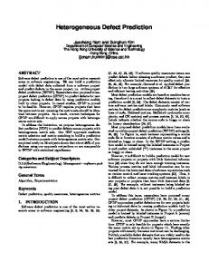
Figure 1: Example of an effort-based cumulative lift chart [48]. Note that, following the practices of Yang et al., we measure Precision, Recall, F1 at the effort = 20% point. The last evaluation metric used in this study is Popt , which is defined as 1 − ∆opt , where ∆opt is the area between the effort (codechurn-based) cumulative lift charts of the optimal model and the prediction model (as shown in Figure 1). In this chart, the x-axis is considered as the percentage of required effort to inspect the change and the y-axis is the percentage of defect-introducing change found in the selected change. In the optimal model, all the changes are sorted by the actual defect density in descending order, while for the predicted model, all the changes are sorted by the actual predicted value in descending order. According to Kamei et al. and Xu et al. [18, 34, 48], Popt can be normalized as follows: S(optimal) − S(m) Popt (m) = 1 − S(optimal) − S(worst) where S(optimal), S(m) and S(worst) represent the area of curve under the optimal model, predicted model, and worst model, respectively. Note that the worst model is built by sorting all the changes according to the actual defect density in ascending order. For any learner, it performs better than random predictor only if the Popt is greater than 0.5.

FSE’2017, September 2017, PADERBORN, GERMANY As similar to the above three evaluation metrics, Precision, Recall, F1, we use 20% of all effort when computing Popt , which is consistent to Yang et al.’s work [48]. Note that in this study, in addition to Popt and ACC (i.e., Recall) that used in Yang et al’s work [48], we include Precision and F1 measures and they provide more insights about all the learners evaluated in the study from very different perspectives, which will be shown in the next section.

6

EMPIRICAL RESULTS

In this section, we present the experimental results to investigate how simple unsupervised learners work in practice and evaluate the performance of the proposed method, OneWay, compared with supervised and unsupervised learners. Before we start off, we need a sanity check to see if we can fully reproduce Yang et al.’s results. Yang et al. [48] provide the median values of Popt and Recall for the EALR model and the best two unsupervised models, LT and AGE, from time-wise cross evaluation experiment. Therefore, we use those numbers to check our results. As shown in Table 3 and Table 4, for unsupervised learners, LT and AGE, we get the exact same performance scores on all projects in terms of Recall and Popt . This is reasonable because unsupervised learners are very straightforward and easy to implement. For the supervised learner, EALR, these two implementations do not have differences in Popt , while the maximum difference in Recall is only 0.02. Since the differences are quite small, then we believe that our implementation reflect the details about EALR and unsupervised learners in Yang et al. [48]. For other supervised learners used in this study, like J48, IBk, and Random Forests, we use the same algorithms from Weka package [10] and set the same parameters as used in Yang et al. [48].

Table 3: Comparison in Popt : Yang’s method (A) vs. our implementation (B) EALR LT AGE Project A B A B A B Bugzilla 0.59 0.59 0.72 0.72 0.67 0.67 Platform 0.58 0.58 0.72 0.72 0.71 0.71 0.50 0.50 0.65 0.65 0.64 0.64 Mozilla JDT 0.59 0.59 0.71 0.71 0.68 0.69 Columba 0.62 0.62 0.73 0.73 0.79 0.79 PostgreSQL 0.60 0.60 0.74 0.74 0.73 0.73 Average 0.58 0.58 0.71 0.71 0.70 0.70

Table 4: Comparison in Recall implementation (B) EALR Project A B Bugzilla 0.29 0.30 Platform 0.31 0.30 Mozilla 0.18 0.18 JDT 0.32 0.34 Columba 0.40 0.42 PostgreSQL 0.36 0.36 Average 0.31 0.32

: Yang’s method (A) vs. our LT A B 0.45 0.45 0.43 0.43 0.36 0.36 0.45 0.45 0.44 0.44 0.43 0.43 0.43 0.43

AGE A B 0.38 0.38 0.43 0.43 0.28 0.28 0.41 0.41 0.57 0.57 0.43 0.43 0.41 0.41

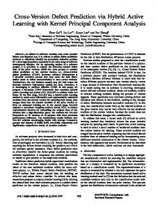
Wei Fu, Tim Menzies RQ1: Do all unsupervised predictors perform better than supervised predictors? To answer this question, we build four supervised learners and twelve unsupervised learners on the six project data sets using incremental learning method as described in Section 5.3. Figure 2 and Figure 3 shows the boxplot of Recall, Popt , F1 and Precision for supervised learners and unsupervised learners on all data sets. For each learner, the boxplot shows the 25th percentile, median and 75 percentile values for one data set. The horizontal dashed lines indicate the median of best supervised learners, which is to help visualize the median differences between unsupervised learners and supervised learners. The colors of the boxes within Figure 2 and Figure 3 indicate the significant difference between learners: • The blue color represents that the corresponding learner is significantly better than the best supervised learner according to Wilcoxon signed-rank, where the BH corrected p-value is less than 0.05 and the magnitude of the difference between these two learners is NOT trivial according to Cliff’s delta, where |δ | ≥ 0.147. • The black color represents that the corresponding learner is not significantly better than the best supervised learner or the magnitude of the difference between these two learners is trivial, where |δ | ≤ 0.147. • The red color represents that the corresponding learner is significantly worse than the best supervised learner and the magnitude of the difference between these two learners is NOT trivial. From Figure 2 and Figure 3, we can clearly see that not all unsupervised learners perform statistically better than the best supervised learner across all different evaluation metrics. Specifically, for Re2 , 3 , 6 , 2 , 3 and 2 of all call, on one hand, there are only 12 12 12 12 12 12 unsupervised learners that perform statistically better than the best supervised learner on six data sets, respectively. On the other hand, 6 , 6 , 4 , 6 , 5 and 6 of all unsupervised learners there are 12 12 12 12 12 12 perform statistically worse than the best supervised learner on the six data sets, respectively. This indicates that: • About 50% unsupervised learners perform worse than the best supervised learner on any data set; • Without any prior knowledge, we can not know which unsupervised learner(s) works adequately on the testing data. Note that the above two points from Recall also hold for Popt . For F1, our observation is that only LT on Bugzilla and AGE on PostgreSQL perform statistically better than the best supervised learner. Other than that, no unsupervised learner performs better on any data set. Furthermore, surprisingly, no unsupervised learner works significantly better than the best supervised learner on any data sets in terms of Precision. As we can see, Random Forests performs well on all six data sets. This suggests that unsupervised learners have very low precision for effort-aware defect prediction and can not be deployed to any business situation where precision is critical. Overall, for a given data set, no one specific unsupervised learner works better than the best supervised learner across all evaluation metrics. For a given evaluation measure, most unsupervised learners did not perform better across all data sets. In summary:

Revisiting Unsupervised Learning for Defect Prediction Recall Unsupervised

Recall

LR RF J48

IBk

NS

ND

y NF ntrop LT E

V P P E P C FIX NDE AG EX REX SEX NU

Popt Supervised

0.0 0.6 0.0 0.6 0.0 0.6 0.0 0.6 0.0 0.6 0.0 0.6

0.0 0.6 0.0 0.6 0.0 0.6 0.0 0.6 0.0 0.6 0.0 0.6

Supervised

EA

FSE’2017, September 2017, PADERBORN, GERMANY

Unsupervised

Popt

LR RF J48

EA

IBk

NS

ND

y NF ntrop LT E

V P P E P C FIX NDE AG EX REX SEX NU

Figure 2: Recall and Popt results. Comparing supervised and unsupervised learners over six projects (from top to bottom are Bugzilla, Platform, Mozilla, JDT, Columba, PostgreSQL). F1 Unsupervised

F1

LR RF J48

EA

IBk

NS

ND

y NF ntrop LT E

V P P E P C FIX NDE AG EX REX SEX NU

Precision Unsupervised

Supervised

0.0 0.6 0.0 0.6 0.0 0.6 0.0 0.6 0.0 0.6 0.0 0.6

0.0 0.6 0.0 0.6 0.0 0.6 0.0 0.6 0.0 0.6 0.0 0.6

Supervised

Precision

LR RF J48

EA

IBk

NS

ND

y NF ntrop LT E

V P P E P C FIX NDE AG EX REX SEX NU

Figure 3: F1 and Precision results. Comparing supervised and unsupervised learners over six projects (from top to bottom are Bugzilla, Platform, Mozilla, JDT, Columba, PostgreSQL).

Not all unsupervised learners perform better than supervised learners for each project and for different evaluation measures. Note the implications of this finding: some extra knowledge is required to prune the unsupervised models, such as the knowledge that comes from labelled data. Hence, we must conclude the opposite to Yang et al.; i.e. some supervised labelled data must be applied before we can reliably deploy unsupervised defect predictors. RQ2: Is it beneficial to use supervised data to prune away most of the Yang et al. models?

To answer this question, we compare the OneWay learner with all twelve unsupervised learners. All these learners are tested on the six project data sets using the same experiment scheme as we did in RQ1. Figure 4 shows the boxplot for the performance distribution of unsupervised learners and the proposed OneWay learner on six data sets across four evaluation measures. The horizontal dashed line denotes the median value of OneWay. Note that in Figure 5, blue means this learner is statistically better than OneWay, red means worse, and black means no difference. As we can see, in Recall, only one unsupervised learner, LT, outperforms OneWay in 46 data sets. 9 , 9 , 9 , 10 , 8 and However, OneWay significantly outperform 12 12 12 12 12

FSE’2017, September 2017, PADERBORN, GERMANY

LT FIX DEV GE EXP EXP EXP UC A N S R N

On

0.0 0.4 0.0 0.4 0.0 0.4 0.00

y NS ND NF trop En

Proposed

LT FIX DEV GE EXP EXP EXP UC A N S R N Precision Unsupervised

ay eW

On

Proposed

0.20 0.0 0.4 0.0 0.6

Proposed

0.20 0.0 0.4 0.0 0.6

F1 Unsupervised

ay eW

0.0 0.6 0.0 0.6 0.0 0.6 0.0 0.6 0.0 0.6 0.0 0.6

y NS ND NF trop En

Popt Unsupervised

Proposed

y NS ND NF trop En

LT FIX DEV GE EXP EXP EXP UC A N S R N

ay eW

On

0.0 0.4 0.0 0.4 0.0 0.4 0.00

0.0 0.6 0.0 0.6 0.0 0.6 0.0 0.6 0.0 0.6 0.0 0.6

Recall Unsupervised

Wei Fu, Tim Menzies

y NS ND NF trop En

LT FIX DEV GE EXP EXP EXP UC A N S R N

ay eW

On

Figure 4: Performance comparisons between the proposed OneWay learner and unsupervised learners over six projects (from top to bottom are Bugzilla, Platform, Mozilla, JDT, Columba, PostgreSQL).

10 12

of total unsupervised learners on six data sets, respectively. This observation indicates that OneWay works significantly better than almost all learners on all 6 data sets in terms of Recall. Similarly, we observe that only LT learner works better than OneWay in 36 data sets in terms of Popt and AGE outperforms OneWay only on platform data set. For the remaining experiments, OneWay perform better than all the other learners (on average, 9 out of 12 learners). In addition, according to F1, only three unsupervised learners EXP/REXP/SEXP perform better than OneWay on Mozilla data set and LT learner just perform as well as OneWay (and has no advantage over OneWay). We note that similar findings can be observed in Precision measure.

Table 5 provides the median values of the best unsupervised learner with OneWay for each evaluation measure on all six data sets. In that table, for each evaluation measure, the number in green background indicates that the best unsupervised learner has a large advantage over OneWay according to the Cliff’s δ ; Similarly, the yellow background means medium advantage and the gray background means small advantage. From Table 5, we observe that out of 24 experiments on all evaluation measures, none of these best unsupervised learners outperform OneWay with a large advantage according to the Cliff’s δ . Specifically, according to Recall and Popt , even though the best unsupervised learner, LT, outperforms OneWay on four and three data sets, all of these advantage are small. Meanwhile, REXP and

LR RF J48 IBk

y Wa

Popt

LR RF J48 IBk

EA

e On

F1 Supervised

Proposed

ay eW

On

0.0 0.6 0.0 0.6 0.0 0.6 0.0 0.6 0.0 0.6 0.0 0.6

Recall

EA

Popt Supervised

Proposed

0.0 0.6 0.0 0.6 0.0 0.6 0.0 0.6 0.0 0.6 0.0 0.6

0.0 0.6 0.0 0.6 0.0 0.6 0.0 0.6 0.0 0.6 0.0 0.6

Recall Supervised

FSE’2017, September 2017, PADERBORN, GERMANY

F1

LR RF J48 IBk

EA

Precision Supervised Proposed

Proposed

ay eW

On

0.0 0.6 0.0 0.6 0.0 0.6 0.0 0.6 0.0 0.6 0.0 0.6

Revisiting Unsupervised Learning for Defect Prediction

Precision

LR RF J48 IBk

EA

ay eW

On

Figure 5: Performance comparisons between the proposed OneWay learner and supervised learners over six projects (from top to bottom are Bugzilla, Platform, Mozilla, JDT, Columba, PostgreSQL).

Table 5: Best unsupervised learner (A) vs. OneWay (B). The colorful cell indicates the size effect: green for large; yellow for medium; gray for small. Project Bugzilla Platform Mozilla JDT Columba PostgreSQL Average

Recall A (LT) B 0.45 0.36 0.43 0.41 0.36 0.33 0.45 0.42 0.44 0.56 0.43 0.44 0.43 0.42

Popt A (LT) 0.72 0.72 0.65 0.71 0.73 0.74 0.71

B 0.65 0.69 0.62 0.70 0.76 0.74 0.69

F1 A (REXP) 0.33 0.16 0.10 0.18 0.23 0.24 0.21

B 0.35 0.17 0.08 0.18 0.32 0.29 0.23

Precision A (EXP) B 0.40 0.39 0.14 0.11 0.06 0.04 0.15 0.12 0.24 0.25 0.25 0.23 0.21 0.19

EXP have a medium improvement over OneWay on one and two data sets for F1 and Precision, respectively. In terms of the average scores, the maximum magnitude of the difference between the best unsupervised learner and OneWay is 0.02. In other words, OneWay is comparable with the best unsupervised learners on all data sets for all evaluation measures. Overall, we find that (1) no one unsupervised learner significantly outperforms OneWay on all data sets for a given evaluation measure; (2) mostly, OneWay works as well as the best unsupervised learner and has significant better performance than almost all unsupervised learners on all data sets for all evaluation measures. Therefore, the above results suggest: As a simple supervised learner, OneWay has competitive performance and it performs better than most unsupervised learners for effort-aware JIT defect prediction. Note the implications of this finding: the supervised learning utilized in OneWay can significantly outperform the unsupervised models.

RQ3: Does OneWay perform better than more complex standard supervised learners? To answer this question, we compare OneWay learner with four supervised learners, including EALR, Random Forests, J48 and IBk. EALR is considered to be state-of-the-art learner for effort-aware JIT defect prediction [18, 48] and all the other three learners are widely used in defect prediction literature over past years [6, 7, 11, 18, 26, 45]. We evaluate all these learners on the six project data sets using the same experiment scheme as we did in RQ1. From Figure 5, we have the following observations. Firstly, the performance of OneWay is significantly better than all these four supervised learners in terms of Recall and Popt on all six data sets. Also, EALR works better than Random Forests, J48 and IBk, which is consistent with Kamei et al’s finding [18]. Secondly, according to F1, Random Forests and IBk perform slightly better than OneWay in two out of six data sets. For most cases, OneWay has a similar performance to these supervised learners and there is no much difference between them. However, when reading Precision scores, we find that, in most cases, supervised learners perform significantly better than OneWay. Specifically, Random Forests, J48 and IBk outperform OneWay on all data sets and EALR is better on three data sets. This finding is consistent to the observation in RQ1 where all unsupervised learners perform worse than supervised learners for Precision. From Table 6, we have the following observation. First of all, in terms of Recall and Popt , the maximum difference in median values between EALR and OneWay are 0.15 and 0.14, respectively, which are 83% and 23% improvements over 0.18 and 0.60 on Mozilla and PostgreSQL data sets. For both measures, OneWay improves the average scores by 0.1 and 0.11, which are 31% and 19% improvement over EALR. Secondly, according to F1, IBk outperforms OneWay on three data sets with a large, medium and small advantage, respectively. The largest difference in median is 0.1. Finally, as we

FSE’2017, September 2017, PADERBORN, GERMANY

Wei Fu, Tim Menzies

Table 6: Best supervised learner (A) vs. OneWay (B). The colorful cell indicates the size effect: green for large; yellow for medium; gray for small. Project Bugzilla Platform Mozilla JDT Columba PostgreSQL Average

Recall A (EALR) 0.30 0.30 0.18 0.34 0.42 0.36 0.32

B 0.36 0.41 0.33 0.42 0.56 0.44 0.42

Popt A (EALR) 0.59 0.58 0.50 0.59 0.62 0.60 0.58

B 0.65 0.69 0.62 0.70 0.76 0.74 0.69

F1 A (IBk) 0.30 0.23 0.18 0.22 0.24 0.21 0.23

B 0.35 0.17 0.08 0.18 0.32 0.29 0.23

Precision A (RF) B 0.59 0.39 0.38 0.11 0.27 0.04 0.31 0.12 0.50 0.25 0.69 0.23 0.46 0.19

discussed before, the best supervised learner for Precision, Random Forests, has a very large advantage over OneWay on all data sets. The largest difference is 0.46 on PostgreSQL data set. Overall, according to the above analysis, we conclude that: OneWay performs significantly better than all four supervised learners in terms of Recall and Popt ; It performs just as well as other learners for F1. As for Precision, other supervised learners outperform OneWay. Note the implications of this finding: simple tools like OneWay perform adequately but for all-around performance, more sophisticated learners are recommended.

7

THREATS TO VALIDITY

In this section, we discuss the potential factors that might threat our results. Internal Validity. The internal validity is related to uncontrolled aspects that may affect the experimental results. One threat to the internal validity is how well our implementation of unsupervised learners could represent the Yang et al.’s method. To mitigate this threat, based on Yang et al “R”code, we strictly follow the approach described in Yang et al’s work and test our implementation on the same data sets as in Yang et al. [48]. By comparing the performance scores, we find that our implementation can generate the same results. Therefore, we believe we can avoid this threat. External Validity. The external validity is related to the possibility to generalize our results. Our observations and conclusions from this study may not be generalized to other software projects. In this study, we use six widely used open source software project data as the subject. As all these software projects are written in java, we can not guarantee that our findings can be directly generalized to other projects, specifically to the software that implemented in other programming languages. Therefore, the future work might include verify our findings on other software project. In this work, we used the data sets from [18, 48], where totally 14 change metrics were extracted from the software projects. We build and test the OneWay learner on those metrics as well. However, there might be some other metrics that not measured in these data sets that work well as indicators for defect prediction. For example, when the change was committed (e.g., morning, afternoon or evening), functionality of the the files modified in this change (e.g., core functionality or not). Those new metrics that are not explored in this study might improve the performance of our OneWay learner.

8

CONCLUSION AND FUTURE WORK

In this paper, we replicate and refute Yang et al.’s results [48] about unsupervised learners for effort-ware just-in-time defect prediction. We find that not all unsupervised learners work better than supervised learners on all six data sets for different evaluation measures. This suggests that we can not randomly pick any one unsupervised learner to perform effort-ware JIT defect prediction. Also reporting results which is aggregated over all projects is discouraged since looking at project-specific results can be very beneficial. Hence, it is necessary to figure out how to pick the best models before deploying them to a project. For that task, supervised learners like OneWay are useful to automatically select the potential best model. In the above, OneWay peformed very well for Recall, Popt and F1. Hence, it must be asked: “Is defect prediction inherently simple? And does it need anything other than OneWay?”. In this context, it is useful to recall that OneWay’s results for precision were not competitive. Hence we say, that if learners are to be deployed in domains where precision is critical, then OneWay is too simple. This study opens the new research direction of applying simple supervised techniques to perform defect prediction. As shown in this study as well as Yang et al.’s work [48], instead of using traditional machine learning algorithms like J48 and Random Forests, simply sorting data according to one metric can be a good defect predictor model, at least for effort-ware just-in-time defect prediction. Therefore, we recommend the future defect prediction research should focus more on simple techniques. For the future work, we plan to extend this study on other software projects, especially those developed by the other programming languages. After that, we plan to investigate new change metrics to see if that helps improve OneWay’s performance.

REFERENCES [1] Fumio Akiyama. 1971. An Example of Software System Debugging.. In IFIP Congress (1), Vol. 71. 353–359. [2] Erik Arisholm and Lionel Briand. 2006. Predicting fault-prone components in a java legacy system. ISESE ’06: Proceedings of the 2006 ACM/IEEE international symposium on International symposium on empirical software engineering (Sep 2006). DOI:http://dx.doi.org/10.1145/1159733.1159738 [3] Yoav Benjamini and Yosef Hochberg. 1995. Controlling the false discovery rate: a practical and powerful approach to multiple testing. Journal of the royal statistical society. Series B (Methodological) (1995), 289–300. [4] Shyam R Chidamber and Chris F Kemerer. 1994. A metrics suite for object oriented design. IEEE Transactions on software engineering 20, 6 (1994), 476–493. [5] Marco D’Ambros, Michele Lanza, and Romain Robbes. 2010. An extensive comparison of bug prediction approaches. In Mining Software Repositories (MSR), 2010 7th IEEE Working Conference on. IEEE, 31–41. [6] Wei Fu, Tim Menzies, and Xipeng Shen. 2016. Tuning for software analytics: Is it really necessary? Information and Software Technology 76 (2016), 135–146. [7] Takafumi Fukushima, Yasutaka Kamei, Shane McIntosh, Kazuhiro Yamashita, and Naoyasu Ubayashi. 2014. An empirical study of just-in-time defect prediction using cross-project models. In Proceedings of the 11th Working Conference on Mining Software Repositories. ACM, 172–181. [8] Todd L Graves, Alan F Karr, James S Marron, and Harvey Siy. 2000. Predicting fault incidence using software change history. IEEE Transactions on software engineering 26, 7 (2000), 653–661. [9] Philip J Guo, Thomas Zimmermann, Nachiappan Nagappan, and Brendan Murphy. 2010. Characterizing and predicting which bugs get fixed: an empirical study of Microsoft Windows. In Software Engineering, 2010 ACM/IEEE 32nd International Conference on, Vol. 1. IEEE, 495–504. [10] Mark Hall, Eibe Frank, Geoffrey Holmes, Bernhard Pfahringer, Peter Reutemann, and Ian H Witten. 2009. The WEKA data mining software: an update. ACM SIGKDD explorations newsletter 11, 1 (2009), 10–18. [11] Tracy Hall, Sarah Beecham, David Bowes, David Gray, and Steve Counsell. 2012. A systematic literature review on fault prediction performance in software

Revisiting Unsupervised Learning for Defect Prediction engineering. IEEE Transactions on Software Engineering 38, 6 (2012), 1276–1304. [12] Maurice Howard Halstead. 1977. Elements of software science. Vol. 7. Elsevier New York. [13] M. Hamill and K. Goseva-Popstojanova. 2009. Common Trends in Software Fault and Failure Data. IEEE Transactions on Software Engineering 35, 4 (July 2009), 484–496. DOI:http://dx.doi.org/10.1109/TSE.2009.3 [14] Ahmed E Hassan. 2009. Predicting faults using the complexity of code changes. In Proceedings of the 31st International Conference on Software Engineering. IEEE Computer Society, 78–88. [15] Tian Jiang, Lin Tan, and Sunghun Kim. 2013. Personalized Defect Prediction. In IEEE/ACM International Conference on Automated Software Engineering. IEEE. [16] Xiao-Yuan Jing, Shi Ying, Zhi-Wu Zhang, Shan-Shan Wu, and Jin Liu. 2014. Dictionary learning based software defect prediction. In Proceedings of the 36th International Conference on Software Engineering. ACM, 414–423. [17] Dennis Kafura and Geereddy R. Reddy. 1987. The use of software complexity metrics in software maintenance. IEEE Transactions on Software Engineering 3 (1987), 335–343. [18] Yasutaka Kamei, Emad Shihab, Bram Adams, Ahmed E Hassan, Audris Mockus, Anand Sinha, and Naoyasu Ubayashi. 2013. A large-scale empirical study of just-in-time quality assurance. IEEE Transactions on Software Engineering 39, 6 (2013), 757–773. [19] Taghi M Khoshgoftaar and Edward B Allen. 2001. MODELING SOFTWARE QUALITY WITH. Recent Advances in Reliability and Quality Engineering 2 (2001), 247. [20] Taghi M Khoshgoftaar and Naeem Seliya. 2003. Software quality classification modeling using the SPRINT decision tree algorithm. International Journal on Artificial Intelligence Tools 12, 03 (2003), 207–225. [21] Taghi M Khoshgoftaar, Xiaojing Yuan, and Edward B Allen. 2000. Balancing misclassification rates in classification-tree models of software quality. Empirical Software Engineering 5, 4 (2000), 313–330. [22] Sunghun Kim, E James Whitehead Jr, and Yi Zhang. 2008. Classifying software changes: Clean or buggy? IEEE Transactions on Software Engineering 34, 2 (2008), 181–196. [23] Sunghun Kim, Thomas Zimmermann, E James Whitehead Jr, and Andreas Zeller. 2007. Predicting faults from cached history. In Proceedings of the 29th international conference on Software Engineering. IEEE Computer Society, 489–498. [24] A G¨unes¸ Koru, Dongsong Zhang, Khaled El Emam, and Hongfang Liu. 2009. An investigation into the functional form of the size-defect relationship for software modules. IEEE Transactions on Software Engineering 35, 2 (2009), 293–304. [25] Taek Lee, Jaechang Nam, DongGyun Han, Sunghun Kim, and Hoh Peter In. 2011. Micro interaction metrics for defect prediction. In Proceedings of the 19th ACM SIGSOFT symposium and the 13th European conference on Foundations of software engineering. ACM, 311–321. [26] Stefan Lessmann, Bart Baesens, Christophe Mues, and Swantje Pietsch. 2008. Benchmarking classification models for software defect prediction: A proposed framework and novel findings. IEEE Transactions on Software Engineering 34, 4 (2008), 485–496. [27] Shinsuke Matsumoto, Yasutaka Kamei, Akito Monden, Ken-ichi Matsumoto, and Masahide Nakamura. 2010. An analysis of developer metrics for fault prediction. In Proceedings of the 6th International Conference on Predictive Models in Software Engineering. ACM, 18. [28] Thomas J McCabe. 1976. A complexity measure. IEEE Transactions on software Engineering 4 (1976), 308–320. [29] Thilo Mende and Rainer Koschke. 2010. Effort-aware defect prediction models. In Software Maintenance and Reengineering (CSMR), 2010 14th European Conference on. IEEE, 107–116. [30] Tim Menzies, Jeremy Greenwald, and Art Frank. 2007. Data mining static code attributes to learn defect predictors. IEEE transactions on software engineering 33, 1 (2007). [31] Tim Menzies, Zach Milton, Burak Turhan, Bojan Cukic, Yue Jiang, and Ays¸e Bener. 2010. Defect prediction from static code features: current results, limitations, new approaches. Automated Software Engineering 17, 4 (2010), 375–407. [32] Ayse Tosun Misirli, Ayse Bener, and Resat Kale. 2011. Ai-based software defect predictors: Applications and benefits in a case study. AI Magazine 32, 2 (2011),

FSE’2017, September 2017, PADERBORN, GERMANY 57–68. [33] Audris Mockus and David M Weiss. 2000. Predicting risk of software changes. Bell Labs Technical Journal 5, 2 (2000), 169–180. [34] Akito Monden, Takuma Hayashi, Shoji Shinoda, Kumiko Shirai, Junichi Yoshida, Mike Barker, and Kenichi Matsumoto. 2013. Assessing the cost effectiveness of fault prediction in acceptance testing. IEEE Transactions on Software Engineering 39, 10 (2013), 1345–1357. [35] Raimund Moser, Witold Pedrycz, and Giancarlo Succi. 2008. A comparative analysis of the efficiency of change metrics and static code attributes for defect prediction. In Proceedings of the 30th international conference on Software engineering. ACM, 181–190. [36] Nachiappan Nagappan and Thomas Ball. 2005. Use of relative code churn measures to predict system defect density. In Software Engineering, 2005. ICSE 2005. Proceedings. 27th International Conference on. IEEE, 284–292. [37] Nachiappan Nagappan, Thomas Ball, and Andreas Zeller. 2006. Mining metrics to predict component failures. In Proceedings of the 28th international conference on Software engineering. ACM, 452–461. [38] Jaechang Nam, Sinno Jialin Pan, and Sunghun Kim. 2013. Transfer defect learning. In Proceedings of the 2013 International Conference on Software Engineering. IEEE Press, 382–391. [39] Thomas J. Ostrand, Elaine J. Weyuker, and Robert M. Bell. 2004. Where the Bugs Are. In Proceedings of the 2004 ACM SIGSOFT International Symposium on Software Testing and Analysis (ISSTA ’04). ACM, New York, NY, USA, 86–96. DOI: http://dx.doi.org/10.1145/1007512.1007524 [40] Thomas J Ostrand, Elaine J Weyuker, and Robert M Bell. 2005. Predicting the location and number of faults in large software systems. IEEE Transactions on Software Engineering 31, 4 (2005), 340–355. [41] Corina S Pasareanu, Peter C Mehlitz, David H Bushnell, Karen Gundy-Burlet, Michael Lowry, Suzette Person, and Mark Pape. 2008. Combining unit-level symbolic execution and system-level concrete execution for testing NASA software. In Proceedings of the 2008 international symposium on Software testing and analysis. ACM, 15–26. [42] Foyzur Rahman, Sameer Khatri, Earl T Barr, and Premkumar Devanbu. 2014. Comparing static bug finders and statistical prediction. In Proceedings of the 36th International Conference on Software Engineering. ACM, 424–434. [43] Jeanine Romano, Jeffrey D Kromrey, Jesse Coraggio, Jeff Skowronek, and Linda Devine. 2006. Exploring methods for evaluating group differences on the NSSE and other surveys: Are the t-test and Cohenfisd indices the most appropriate choices. In annual meeting of the Southern Association for Institutional Research. [44] Forrest Shull, Ioana Rus, and Victor Basili. 2001. Improving Software Inspections by Using Reading Techniques. In Proceedings of the 23rd International Conference on Software Engineering (ICSE ’01). IEEE Computer Society, Washington, DC, USA, 726–727. http://dl.acm.org/citation.cfm?id=381473.381612 [45] Burak Turhan, Tim Menzies, Ays¸e B Bener, and Justin Di Stefano. 2009. On the relative value of cross-company and within-company data for defect prediction. Empirical Software Engineering 14, 5 (2009), 540–578. [46] Song Wang, Taiyue Liu, and Lin Tan. 2016. Automatically learning semantic features for defect prediction. In Proceedings of the 38th International Conference on Software Engineering. ACM, 297–308. [47] Maurice V Wilkes. 1985. Memoirs ofa Computer Pioneer. Cambridge, Mass., London (1985). [48] Yibiao Yang, Yuming Zhou, Jinping Liu, Yangyang Zhao, Hongmin Lu, Lei Xu, Baowen Xu, and Hareton Leung. 2016. Effort-aware just-in-time defect prediction: simple unsupervised models could be better than supervised models. In Proceedings of the 2016 24th ACM SIGSOFT International Symposium on Foundations of Software Engineering. ACM, 157–168. [49] Zuoning Yin, Ding Yuan, Yuanyuan Zhou, Shankar Pasupathy, and Lakshmi Bairavasundaram. 2011. How do fixes become bugs?. In Proceedings of the 19th ACM SIGSOFT symposium and the 13th European conference on Foundations of software engineering. ACM, 26–36. [50] Thomas Zimmermann, Rahul Premraj, and Andreas Zeller. 2007. Predicting defects for eclipse. In Proceedings of the third international workshop on predictor models in software engineering. IEEE Computer Society, 9.