MANUAL TRAINING AND SYSTEM IDENTIFICATION. Roberto Iglesias1, Theocharis Kyriacou2, Ulrich Nehmzow2 and Steve Billings3. 1 Dept. of Electronics ...
ROBOT PROGRAMMING THROUGH A COMBINATION OF MANUAL TRAINING AND SYSTEM IDENTIFICATION Roberto Iglesias1 , Theocharis Kyriacou2 , Ulrich Nehmzow2 and Steve Billings3 1
Dept. of Electronics and Computer Science, University of Santiago de Compostela, Spain 2 Dept. of Computer Science, University of Essex, Colchester.UK 3 Dept. of Automatic Control/Syst. Eng., University of Sheffield, Sheffield, UK ABSTRACT
In this paper we present a novel procedure to obtain the control code for a mobile robot executing sensor-motor tasks. The process works in two stages: First, the robot is controlled by a human operator who manually guides the robot through the sensor-motor task. The robot’s motion is then “identified”, using the NARMAX system identification technique. This process, which we refer to as RobotMODIC (robot modelling, identification and characterisation) has distinct advantages over existing robot programming techniques: 1. The RobotMODIC process allows very rapid code development without the need of iterative refinement, 2. it requires little a priori knowledge of the task performed — the robot is merely driven manually during the training phase, 3. the RobotMODIC process produces extremely compact code, 4. the generated coupling between perception and action can be analysed, using mathematical methods, and 5. the generated code is largely robot-platform independent. The RobotMODIC process represents a step towards a science of mobile robotics, because it reveals fundamental properties of the sensor-motor couplings underlying the robot’s behaviour through its transparent and analysable modelling method. 1. INTRODUCTION Industrial and technical applications of sensor-response systems (such as mobile robots) are continuously gaining importance, in particular under considerations of reliability (uninterrupted and reliable execution of monotonous tasks such as surveillance), accessibility (inspection of sites that
are inaccessible to humans), and cost (transportation systems based on autonomous mobile robots are more flexible and can be cheaper than standard track-bound systems). Mobile robots are already widely used for surveillance, inspection and transportation tasks. Fundamentally, the behaviour of a robot is influenced by three components: i) the robot’s hardware, ii) the program it is executing, and iii) the environment the robot is operating in. It is a common experience in robotics that a robot program written with a specific task in mind almost never produces the desired behaviour straight away. Instead, iterative refinement is used: a good first guess at a feasible control strategy is implemented, then tested in the target environment. If the robot fails to solve the task, the control code is refined, and the process is repeated until the specific task is successfully completed in the target environment. Such an existence proof demonstrates that a particular robot can achieve a particular task under a particular set of environmental conditions, but says little about the program’s dependency upon specific environmental conditions. Such knowledge is desirable, though, because it is relevant to issues such as scaling or operation under modified environmental conditions. In this paper we therefore propose a novel procedure to program a robot controller, based on system identification techniques [1, 2]. Instead of refining an initial approximation of the desired control code through a process of trial and error, we identify — determine the relevant inputoutput parameters of the robot control process — the motion of a manually, “perfectly” driven robot, and subsequently use the result of the identification process to achieve autonomous robot operation. While the robot is being remotely controlled we log sufficient information to model the relationship between the robot’s sensor perception and motor response, using a nonlinear polynomial function. This function can be used afterwards during autonomous operation to determine the translational and rotational velocities that are suitable for the desired behaviour. There are important benefits from the procedure we pro-
pose in this article. First, the process is fast and requires little a priori knowledge about the desired robot behaviour, because the robot is manually, “perfectly” guided through the desired motion. Code development is very fast. Secondly, the developed code is very compact, which is useful for applications where memory and processing speed matter. Thirdly, the obtained control code is transparent, i.e. represented as a function (in our case, a polynomial), which is amenable to mathematical analysis. Finally, in many cases the generated code is platform-independent and can be used without modifications on different robot bases [3]. The process outlined in this paper is part of the RobotMODIC project conducted at the universities of Essex and Sheffield, whose ultimate purpose it is to develop elements of a theory of robot-environment interaction that supports the off-line design of robot controllers, and that makes testable and falsifiable hypotheses about that interaction.
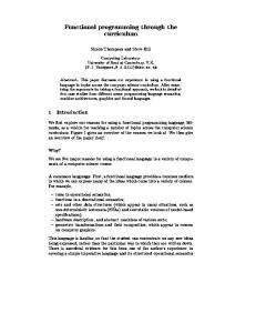
Fig. 2.
E XPERIMENTAL SCENARIO FOR THE DOOR TRAVERSAL BEHAVIOUR . T HE INITIAL POSITIONS OF THE ROBOT WERE WITHIN THE SHADED AREA .
2. EXPERIMENTAL SETUP AND METHOD 2.1. Task and Experimental Procedure Our goal was to “program” a Magellan Pro mobile robot (figure 1) to traverse a door-like opening, making a minimum of initial assumptions and using no pre-installed knowledge. This experimental scenario is shown in figure 2. The Magellan Pro is equipped with front-facing laser, sonar, infrared, tactile and vision sensors. In the experiments reported here we only used the laser, which covers the semicircle in front of the robot, and the sixteen omni-directional sonar sensors of the robot.
Fig. 1. R ADIX ,
THE OUR EXPERIMENTS .
M AGELLAN P RO
ROBOT USED IN
The opening the robot had to traverse had a width of
two robot diameters (80 cm), the robot’s starting positions for both training and testing data were selected to lie in the shaded area indicated in figure 2, between 1.2m and 3m from the opening. The task of “door traversal” is a relatively complex sensor-motor task, because the robot’s motion has to be controlled carefully in order to avoid collisions, and because different sensor signals have to be used at different stages of the process: as the robot approaches a door from afar, the door is only visible to the laser sensors. In the vicinity of the door, both laser and sonar sensors can detect it, whilst only the sonar sensors can detect the door once the robot is traversing it, because the laser sensors only cover the semicircle ahead of the robot. To achieve this door traversal task, we moved the robot manually, controlling it from a remote computer. During the manual operation of the robot, we logged sensor and position information every 250 ms, using an overhead camera logging system. After the collection of experimental data, a Non-linear Auto-Regressive Moving Average model with eXogenous inputs (NARMAX) was estimated ([4], see next section). This model relates robot sensor values to actuator signals. An interesting aspect of the approach taken is that we did not attempt to identify “useful” sensors beforehand — we constructed a model, using all available sensor information, and used the model itself to detect which sensor signals carry meaningful information with respect to the door traversal task. 2.2. NARMAX modelling The NARMAX modelling approach is a parameter estimation methodology for identifying both the important model
terms and the parameters of unknown non-linear dynamic systems. For multiple input, single output noiseless systems this model takes the form: y(n)
=
f (u1 (n), u1 (n − 1), u1 (n − 2), · · · , u1 (n − Nu ), u1 (n)2 , u1 (n − 1)2 , u1 (n − 2)2 , · · · , u1 (n − Nu )2 , ··· , u1 (n)l , u1 (n − 1)l , u1 (n − 2)l , · · · , u1 (n − Nu )l , u2 (n), u2 (n − 1), u2 (n − 2), · · · , u2 (n − Nu ), u2 (n)2 , u2 (n − 1)2 , u2 (n − 2)2 , · · · , u2 (n − Nu )2 , ··· , u2 (n)l , u2 (n − 1)l , u2 (n − 2)l , · · · , u2 (n − Nu )l , ··· , ··· , ud (n), ud (n − 1), ud (n − 2), · · · , ud (n − Nu ), ud (n)2 , ud (n − 1)2 , ud (n − 2)2 , · · · , ud (n − Nu )2 , ··· , ud (n)l , ud (n − 1)l , ud (n − 2)l , · · · , ud (n − Nu )l , y(n − 1), y(n − 2), · · · , y(n − Ny ), y(n − 1)2 , y(n − 2)2 , · · · , y(n − Ny )2 , ··· , y(n − 1)l , y(n − 2)l , · · · , y(n − Ny )l )
were y(n) and u(n) are the sampled output and input signals at time n respectively, Ny and Nu are the regression orders of the output and input respectively and d is the input dimension. f () is a non-linear function and it is typically taken to be a polynomial or wavelet multi-resolution expansion of the arguments. The degree l of the polynomial is the highest sum of powers in any of its terms. The NARMAX methodology breaks the modelling problem into the following steps: i) Structure detection, ii) parameter estimation, iii) model validation, iv) prediction, and v) analysis. A detailed procedure of how these steps are done is presented in [5, 4, 6], nevertheless a brief explanation of them is given below. Any data set that we intend to model is first split in two sets (usually of equal size). The first, referred to as the estimation data set, is used to calculate the model parameters. The remaining data set, referred to as the validation set, is used to test and evaluate the model. The structure of the NARMAX polynomial is determined by the inputs u, the output y, the input and output orders Nu and Ny respectively and the degree l of the polynomial. The number of terms of the NARMAX model polynomial can be very large depending on these variables, but not all of them are significant contributors to the computation of the output, in fact often most terms can be safely removed from the model equation without this introducing any significant errors.
The calculation of the NARMAX model parameters is an iterative process. Each iteration involves three steps: i) estimation of model parameters, ii) model validation and iii) removal of non-contributing terms. In the first step the NARMAX model is used to compute an equivalent auxiliary model whose terms are orthogonal, thus allowing their associated parameters to be calculated sequentially and independently from each other. Once the parameters of the auxiliary model are obtained, the NARMAX model parameters are computed from the auxiliary model. The NARMAX model is then tested using the validation data set. If the error between the model predicted output and the actual output is below a user-defined threshold, noncontributing model terms are removed in order to reduce the size of the polynomial. To determine the contribution of a model term to the output, the so-called Error Reduction Ratio (ERR) [4] is computed for each term. The ERR of a term is the percentage reduction in the total mean-squared error (i.e. the difference between model predicted and true system output) as a result of including (in the model equation) the term under consideration. The bigger the ERR is, the more significant the term. Model terms with ERR under a certain threshold are removed from the model polynomial. In the following iteration, if the error is higher as a result of the last removal of model terms then these are re-inserted back into the model equation and the model is considered as final. 3. EXPERIMENTAL RESULTS This section presents an example of robot programming through system identification. As stated above, we want to solve the task of door-traversal. First the data collection procedure for this task is explained. After that, we show the model which identifies the robot’s behaviour when it was manually controlled. Finally, a comparison is made between the behaviour of the robot when it is manually controlled and when executing the NARMAX model of the task. 3.1. Door Traversal The task we want to solve with the robot is the door traversal. In this task, usual in robot navigation, the robot has to go towards a door which is close to it, and afterwards it has to cross the door avoiding to collide with the door frame, and keeping its position as centred as possible. In our case the initial position of the robot is chosen to be between 120 cm and 300 cm from the door it has to cross (figure 2), and the size of the door is 80 cm (about twice the robot’s diameter).
In figure 3 we can see the trajectories of the robot after crossing 39 times the same door. The initial position was different each time and the robot was always manually controlled. For simplicity, the value of the translational velocity was constant (0.07 m/s), so that the human operator only controlled the rotational velocity at every instant.
segmentation of data (which generates singularities in the training data) and the fact that the robot does not always turn at the same point make the system identification task hard.
3.2. Data Used for the System Identification Using the procedure described in section 2.2, a model of the door traversal behaviour was then obtained. In order to avoid making assumptions about the relevance of specific sensor signals, all the ultrasound and laser measurements were taken into account. The values delivered by the laser scanner were averaged in twelve sectors of 15 degrees each, to obtain a twelve dimensional vector of laser-distances. Although this was not essential for the modelling process, these laser distances as well as the 16 sonar sensor values, were inverted before they were used to obtain the model, so that large readings indicate close-by objects. The model structure was of input order Nu = 0, output order Ny = 0, and degree l = 2. This initially produced a polynomial of 435 terms of which, after iterative refinement, only 38 remained. The final model equation is shown in table 1.
3.3. Original and model behaviour comparison
Fig. 3. T OP : T HE ROBOT ’ S TRAJECTORIES UNDER MAN UAL CONTROL (39 RUNS , TRAINING DATA ). B OTTOM : T RAJECTORIES TAKEN UNDER MODEL CONTROL (41 RUNS , TEST DATA ). T HE WHITE LINES ON THE FLOOR WHERE USED TO AID THE HUMAN OPERATOR IN SELECTING START LOCATIONS , THEY WERE INVISIBLE TO THE ROBOT. As we can see in figure 3, this is an episodic task, which means that the operation of the robot is naturally divided into independent episodes. The performance in each episode (which comprises the movement of the robot from the starting position to the final position once the door has been crossed), depends only on the actions taken during that episode. Also, figure 3 shows that the robot turns at different angles and distances to the door in different runs. Both the
Figure 3 (bottom), shows the trajectories of the robot when the NARMAX model was used to control it. Door traversal was performed 41 times. The initial positions of the robot during testing were located in the same area as those used for training (see figure 2). Figure 3 reveals some interesting phenomena, stemming from the teaching procedure used. In the first door traversal under human control, the human operator moved the robot towards the centre of the door when the was still far from the opening. This resulted in the jagged trajectories visible in figure 3 (top). As the human operator gained experience, he was able to execute more efficient motions, nearer the door. Figure 3 (bottom) shows how the NARMAX model controlled the robot in a manner that was smooth in all trajectories. To determine the degree of similarity between the trajectories achieved under human control and those observed under automatic control (figure 3), we analysed the trajectories through the door, comparing the x positions the robot occupied when it was at the centre of the opening. These distributions, which indicate the offset from the centre of the door, are shown in figure 4. There is a statistically significant difference between these distributions (U-test, p > 0.05) [7]: the model-driven robot traverses the door more centrally than the human-driven robot.
Frequency 25.0
left side of the door
right side of the door centre of the door
20.8
16.7
˙ = θ(t) +0.272 +0.189 ∗ (1/d1 (t)) −0.587 ∗ (1/d3 (t)) −0.088 ∗ (1/d4 (t)) −0.463 ∗ (1/d6 (t)) +0.196 ∗ (1/d8 (t)) +0.113 ∗ (1/d9 (t)) −1.070 ∗ (1/s9 (t)) −0.115 ∗ (1/s12 (t)) +0.203 ∗ (1/d3 (t))2 −0.260 ∗ (1/d8 (t))2 +0.183 ∗ (1/s9 (t))2 +0.134 ∗ (1/(d1 (t) ∗ d3 (t))) −0.163 ∗ (1/(d1 (t) ∗ d4 (t))) −0.637 ∗ (1/(d1 (t) ∗ d5 (t))) −0.340 ∗ (1/(d1 (t) ∗ d6 (t))) −0.0815 ∗ (1/(d1 (t) ∗ d8 (t))) −0.104 ∗ (1/(d1 (t) ∗ s8 (t))) +0.075 ∗ (1/(d2 (t) ∗ s7 (t))) +0.468 ∗ (1/(d3 (t) ∗ d5 (t))) +0.046 ∗ (1/(d3 (t) ∗ s5 (t))) +0.261 ∗ (1/(d3 (t) ∗ s12 )) +1.584 ∗ (1/(d4 (t) ∗ d6 (t))) +0.076 ∗ (1/(d4 (t) ∗ s4 (t))) +0.341 ∗ (1/(d4 (t) ∗ s12 (t))) −0.837 ∗ (1/(d5 (t) ∗ d6 (t))) +0.360 ∗ (1/(d5 (t) ∗ d7 (t))) −0.787 ∗ (1/(d6 (t) ∗ d9 (t))) +3.145 ∗ (1/(d6 (t) ∗ s9 (t))) −0.084 ∗ (1/(d6 (t) ∗ s13 (t))) −0.012 ∗ (1/(d7 (t) ∗ s15 (t))) +0.108 ∗ (1/(d8 (t) ∗ s3 (t))) −0.048 ∗ (1/(d8 (t) ∗ s6 (t))) −0.075 ∗ (1/(d9 (t) ∗ s4 (t))) −0.105 ∗ (1/(d10 (t) ∗ d12 (t))) −0.051 ∗ (1/(d10 (t) ∗ s12 (t))) +0.074 ∗ (1/(d11 (t) ∗ s1 (t))) −0.056 ∗ (1/(d12 (t) ∗ s7 (t))) Table 1. NARMAX MODEL OF THE ANGULAR VELOC ITY θ˙ FOR THE DOOR TRAVERSAL BEHAVIOUR , AS A FUNCTION OF LASER AND SONAR INFORMATION .
12.5
8.3
4.2
0.0 350
Frequency
360
370
380
390
400
25.0
left side of the door
centre of the door
410
420
x position (in pixels)
right side of the door
20.8
16.7
12.5
8.3
4.2
0.0 350
360
370
380
390
400
410
420
x position (in pixels)
Fig. 4. D ISTRIBUTION OF x POSITION WHEN CROSSING THE DOOR . T RAINING DATA ( ROBOT IS BEING MANU ALLY DRIVEN ) IS SHOWN ON TOP, TESTING DATA ( ROBOT IS BEING DRIVEN BY THE NARMAX MODEL ) BELOW. Scaling Up and Generalisation Finally, figure 5 shows how the model performs in environments different to the training environment. In both environments shown in figure 5 the robot steered through successive doors, without collision and traversing doors centrally. 4. CONCLUSIONS This paper introduces a novel mechanism to program robots through system identification, rather than an empirical trialan-error process of iterative refinement. To achieve sensor-motor tasks, we first operate the robot under human supervision, making it follow a desired trajectory. Once training data is acquired in this way, we use the NARMAX modelling approach to obtain a model which identifies the coupling between sensory perception and motor response as a non-linear polynomial. This model is then used to control the robot when it moves autonomously. A control program obtained in this way is not just an
Acknowledgements The authors thank the following institutions for their support: The RobotMODIC project is supported by the Engineering and Physical Sciences Research Council under grant GR/S30955/01. R.I. is supported through the research grants PGIDIT04TIC206011PR and TIC2003-09400-C0403. 5. REFERENCES [1] Ulrich Nehmzow, Thecharis Kyriacou, Roberto Iglesias, and Steve Billings, “Robotmodic: Modelling, identification and characterisation of mobile robots,” in Proceedings of TAROS 2004 - Towards Autonomous Robotic Systems, 2004. [2] P. Eykhoff, Trends and Progress in System Identification, Pergamon Press, 1981. [3] T. Kyriacou, U. Nehmzow, R. Iglesias, and S. Billings, “Cross-platform programming through system identification,” in Proc. Towards Autonomous Robotic Systems. 2005, Imperial College London. [4] M. Korenberg, S. Billings, Y. P. Liu, and P. J. McIlroy, “Orthogonal parameter estimation algorithm for non-linear stochastic systems,” International Journal of Control, vol. 48, pp. 193–210, 1988.
Fig. 5. T RAJECTORY OF THE ROBOT WHEN THE NARMAX MODEL WAS USED TO CONTROL IT IN AN ENVIRONMENT DIFFERENT FROM THE ONE USED FOR TRAINING .
“existence proof”, in the sense that it shows that the robot can achieve a particular behaviour under particular environmental conditions, but it also allows the analysis of the main factors involved in the robot’s operation in the environment. This knowledge can be used to formulate new justified and testable hypotheses which can lead to a new stage of the experimentation and design of a controller, resulting in a more effective and goal-oriented design process [8]. Our first experimental results confirm that there are cases where the methodology described in this paper is viable. In particular we used our proposal to solve a complex and useful task in mobile robotics (door traversal). The model we obtained was able to move the robot properly and even better than under manual control. The circumstances under which programming through system identification and training is a viable way to proceed in general is subject to ongoing research at the universities of Essex and Sheffield.
[5] S. Billings and S. Chen, “The determination of multivariable nonlinear models for dynamical systems,” in Neural Network Systems, Techniques and Applications, C. Leonides, Ed., pp. 231–278. Academic press, 1998. [6] S. Billings and W. S. F. Voon, “Correlation based model validity tests for non-linear models,” International Journal of Control, vol. 44, pp. 235–244, 1986. [7] C. Barnard, F. Gilber, and P. McGregor, Asking questions in Biology. Design, analysis & presentation in practical Work, Longman Sicientific & Technical, 1993. [8] Roberto Iglesias, Ulrich Nehmzow, Thecharis Kyriacou, and Steve Billings, “Modelling and characterisation of a mobile robot’s operation,” in Proceedings of CAEPIA’05, submitted.