Nicholas Molton, Stephen Se, David Lee, Penny Probert, Michael Brady. Department of Engineering Science. University of Oxford. Parks Road, Oxford OX1 3PJ.
Robotic Sensing for the Guidance of the Visually Impaired Nicholas Molton, Stephen Se, David Lee, Penny Probert, Michael Brady Department of Engineering Science University of Oxford Parks Road, Oxford OX1 3PJ U. K. Abstract This paper describes ongoing work into a portable mobility aid, worn by the visually impaired. The system uses stereo vision and sonar sensors for obstacle avoidance and recognition of kerbs. Because the device is carried, the user is given freedom of movement over kerbs, stairs and rough ground, not traversable with a wheeled aid. Motion of the sensor due to the walking action is measured using a digital compass and inclinometer. This motion has been modelled and is tracked to allow compensation of sensor measurements. The vision obstacle detection method uses comparison of image feature disparity with a ground feature disparity function. The disparity function is continually updated by the walk-motion model and by scene ground-plane fitting. Kerb detection is achieved by identifying clusters of parallel lines using the Hough transform. Experimental results are presented from the vision and sonar parts of the system.
1
Introduction
There are over 40 million visually impaired people worldwide. Mobility aids can support a greater degree of independence, making it possible to travel without a human guide. The most commonly used mobility aids are the long cane and guide dog. The acceptance of these devices has been limited by concerns such as the short range of the cane, the lack of protection against head-height obstacles, and the expense and day-to-day challenges of looking after a dog. Attempts to substitute for the lost sense of vision have included the mapping of camera images straight onto tactile arrays mounted on the skin [Collins, 1985]. This, however, has been found to provide too much detail to the user and the response of the skin soon becomes tired. An alternative which may be practical in a number of years is the connection of cameras to the human nervous system [Dagnelie and Massof, 1996]. While an exciting prospect, this would not be suitable for many people who
are unwilling to undergo surgery or whose visual cortex is damaged. A number of electronic mobility aids using sonar [Russell, 1965; Pressey, 1977; Kay, 1964] have been developed but are not widely used as they give limited useful information or require extensive training. The continuing exponential increase in computer processing power has recently made computer vision a practical technique for feature detection in a mobility aid. This paper describes ongoing work into a portable aid which makes use of both sonar and computer vision. The design goal is to detect obstacles at least 10cm high, at a range of up to 5 metres. The sonar and vision sensors complement each other in several ways. Stereo vision gives precise directional information and uncertain range; sonar measures range precisely but with high angular uncertainty. The vision algorithm can detect small obstacles close to the ground; sonar is more easily confused by reflections from the ground. Transparent objects, such as windows, may be missed by vision, but detected by sonar. There are other aids based on vision under development which use devices on wheels [Mori et al., 1994]. While these allow easy transfer of methods from the field of mobile robotics, we have taken the additional step of removing the device from the ground. This gives a number of important benefits: • The ability to walk naturally, in a manner dictated entirely by the user • Increased mobility(over stairs, hills, kerbs and uneven ground) • Increased travelling speed The project prototype, as shown in Figure 1, comprises system electronics in a backpack and sensors which are mounted either on the backpack or on the user’s body. Three sonar sensors are fixed to the user’s belt and one is mounted at chest height. These sensors are driven and interpreted by a Motorola HC11 microcontroller. Two calibrated greyscale cameras are mounted on rigid arms, which extend over the user’s shoulders from the backpack. The camera orientation can be adjusted over a small range for alignment. The vision part
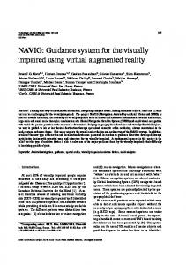
1 0.9
2.5m 3m
0.8
3.5m
4m 4.5m 5m
Probability of Detection
0.7 0.6 0.5 0.4 0.3 0.2 0.1 0 0
2
4
6
8 10 12 Obstacle Size (cm)
14
16
18
20
Figure 2: Obstacle detection probability at various distances. Figure 1: The project prototype. of the project at present uses an image capture and process board based on the TI C40 processor. Section 2 summarises the vision-based Ground-Plane Obstacle Detection (GPOD) algorithm, which uses disparity between stereo image pairs to detect potential obstacles. Obstacle detection is complicated by the significant sensor movements that arise from the user’s walking action. Section 3 describes techniques to measure and predict the motion of the sensors. Section 4 then extends the GPOD algorithm to deal with these movements. Surveys of visually impaired people have reported considerable interest in a mobility aid which could assist in centre-path travel. With this objective, Section 5 presents results in the automatic detection of kerbs. The user interface is a key component of any mobility aid. Section 6 describes the system’s user interface and the tests which have been performed on the sonar part of the system with the help of visually impaired volunteers. Section 7 summarises the work and considers directions for future research.
2
Ground Plane Obstacle Detection
Ground Plane Obstacle Detection (GPOD) using stereo disparity was first reported by Sandini [Ferrari et al., 1990] and subsequently refined by Mayhew [Mayhew et al., 1992] and by Li [Li, 1994; Li et al., 1995]. GPOD uses a pair of cameras to detect features which do not lie on the ground plane. GPOD parameterises the ground plane using measurements of disparity, rather than the depths of world features. This improves robustness to calibration errors. It is a feature-based stereo algorithm. Images of the ground that contain line features but no obstacles are used to initialise the ground plane estimate.
GPOD works in image coordinates, and compares the disparity values in a new image pair with the expected ground plane disparity to detect differences. The measured disparity of an obstacle is significantly larger than that which has been predicted for the ground. Vertical edges are detected using a Sobel detector, and stereo matching uses the PMF algorithm [Pollard et al., 1991a; 1991b]. Special cases of the Sobel and PMF algorithms decrease the cycle time [Li, 1994]. The ground plane disparity d varies linearly with cyclopean image plane position [Li et al., 1995], that is d = au + bv + c
(1)
where (u, v) is the cyclopean image coordinate. In initialisation, a least-squares fit is used to estimate the ground plane parameters (a, b, c). The algorithm has been extended to sub-pixel accuracy by parabolic interpolation during Sobel edge detection and a better fit with lower residue is obtained. As the image coordinates and the measured disparity are not noise-free, a ground plane parameters uncertainty analysis has been carried out [Se and Brady, 1997] to tell us how much confidence we can have in our ground plane estimate. Noise also makes obstacle detection a stochastic process and therefore, reliability measures such as obstacle detection and false alarm are studied in probabilistical terms [Se and Brady, 1998]. We obtain Figure 2 which shows the probability of obstacle detection for different obstacle sizes at various distances.
3
Walker Egomotion Measurement
An estimate of the motion of sensors carried by a walking person is essential if computer vision and sonar sensing are to be useful in this application. An estimate of motion now and in the future is required for three reasons: • To estimate ground position when it cannot be seen
Sensor
Low-pass Filter
Signal Parameter Extractor
Fundamental signal parameters at current time
10 Kalman Filter
Motion Model
Estimation of sensor position as a function of time
5 Roll (degrees)
Motion estimate
Motion estimate
Pattern Detector (stopped,travelling, turning etc)
signal frequency
Figure 3: Measurement process overview.
Wavelet
Measured
0
−5 Wavelet+Kalman Filter
• To removal the complex gait motion from the perceived motion of world entities, to allow tracking • An aid to image feature matching through time It is possible to deduce motion using an intrinsic sensor (one of the system’s object detection sensors; e.g. vision) or an extrinsic sensor (a sensor specifically designed to measure motion; e.g. an accelerometer or gyroscope). In the following sections results from an extrinsic sensor are reported. The principles of using the cameras (intrinsic sensors) to calculate egomotion are described in [Molton et al., 1997]. Experimental analysis of walking gait showed that the components of motion are approximately sinusoidal in form [Lee, 1996]. Each component is therefore modelled by a single sine wave with fundamental signal parameters of amplitude, frequency, phase, and a fixed offset from zero, which are assumed to be constant over short periods of time, and must be estimated as the user walks. A change in the type of motion is detected by a pattern detector and a tracking action chosen accordingly. If, for example, the change in the motion falls below a threshold value, it is assumed that the person has stopped walking and the current position is then used as an estimate of future position. Figure 3 shows a summary of how gait, measured by a motion sensor, might be tracked, and future position predicted.
3.1
Analysing Gait With a Kalman Filter
A digital compass and inclinometer module was used to measure rotation during walking, and allow the motion estimation process to be tested. The motion model outlined in the previous section can be described by: Roll = Ar cos(θr ) + Dr
(2)
P itch = Ap cos(θp ) + Dp (3) Y aw = Ay cos(θy ) + Dy (4) The model assumes nominally fixed frequency, offset, and amplitude. Phase angle (θ) is updated at each step by the state transition matrix, using the frequency estimate. An iterated, extended Kalman Filter [BarShalom and Fortmann, 1988] based on this model was implemented. A sample of predictions made with it for a variable walking speed roll signal are shown in Figure 4.
−10 9.5
10
10.5
11 Time (seconds)
11.5
12
12.5
Figure 4: Roll measured during walking, and a prediction of the measurement made 0.25 seconds earlier using a Kalman filter, wavelets, or both. Because the filter must be flexible enough to change with the measurements, its estimate is imprecise. The root mean square error in the roll prediction for the whole variable walking speed signal was 4.7 degrees. Fundamental problems with using a Kalman filter are that: • The robustness of tracking is limited because a nonlinear system is being linearised. • The system parameters are estimated for the entire history of the signal. In fact, since the parameters are changing in an unmodellable way (meandering) they should be estimated using local data.
3.2
Analysing Gait Using Wavelets
The sinusoidal parameters of the gait motion can also be extracted using wavelets. These are considered because they have the ability to extract instantaneous frequency and phase information from a signal very robustly and accurately [Kovesi, 1996]. Gabor wavelets in quadrature are used for the analysis, over a range of frequencies sufficient to cover the variety of expected walk frequencies. For each frequency, discrete even and odd wavelets, of size ψ, are convolved with the last ψ elements of a particular motion measurement (roll, pitch or yaw). The centre values of these convolutions give the real and imaginary parts of the scalar response to this frequency. The magnitude of this complex number is calculated and the frequency giving highest response is found. The phase of the complex number corresponding to the maximum response gives the phase of the signal at each particular time. The magnitude of the wavelet response also allows calculation of signal amplitude. Predictions of roll for the variable speed walking example are shown in Figure 4. This time the root mean square error in the prediction was 4.8 degrees.
The biggest problem with wavelet analysis is that it estimates the parameters over a region of the signal which can never be zero, resulting in a delay in the signal extraction process. This is a major reason for the error observed in the roll prediction. The derivatives of the measurements may also be examined using wavelets. Linear changes in a signal offset, such as occur in the yaw signal when the walker turns a corner, cannot be dealt with using the wavelet analysis method described. The second derivative of such a signal however does not show any offset and so, if analysed carefully, can be used to give a better result. The disadvantages of the Kalman Filter method and wavelet method can be overcome to some extent by using the results of a wavelet analysis as input to a Kalman Filter. The result of doing this for the variable walking speed example is again shown in Figure 4. This time the root mean square error for the entire signal sample was 4.6 degrees, lower than for the other methods but still significant. This short sample includes a substantial increase in walking speed, which has not yet been detected by the predictor. Most of the prediction error arises from the resulting phase errors in the latter half of the sample.
4
Dynamic Ground Plane Recalibration
For wheeled mobile robots moving over flat ground, there is no change in position of the ground plane relative to the cameras, and the cyclopean ground-plane disparity function is therefore fixed. However, the sensor movements that were modelled in the previous section make it impossible to use a one-time, fixed ground plane calibration in this application. Dynamic recalibration of the ground plane is important: • to prevent human movement affecting obstacle detection. For example, when the height of the cameras reduces a little, with a constant ground plane, the system will deduce the ground plane to be below the ground, thus classifying ground plane features wrongly as obstacles. • to obtain a better estimate of the ground plane for slopes, hills or non-flat ground. For instance, in the case of an uphill slope, with a constant ground plane, the horizontal plane estimate will wrongly classify features on the uphill ground plane as obstacles.
4.1
The Algorithm
The algorithm for Dynamic Ground Plane Recalibration (DGPR) is as follows [Se, 1996; Molton et al., 1997]: Initialization Step1 Use features on the ground plane, with no obstacles, for GPOD calibration, yielding the initial (a, b, c) parameters. Initiate tracks for the features on the ground plane, classified as Type I features.
Normal Step Iteratively, using step k’s ground plane parameters for obstacle detection, partition the features found into 2 types: • Type I for ground plane features; • Type II for obstacle features. Perform track initiation, maintenance and termination for features of each type. Use the new Type I features and motion estimate (from the work of Section 3) to obtain step k + 1’s ground plane parameters. Use Type II features information to send alarms to the user about nearby frontal obstacles. The camera motion estimate required for the prediction of ground plane parameters in the next frame is difficult to obtain accurately over long periods and does not react to changes in ground slope [Molton, 1996]. Therefore, when many ground features can be seen, we use ground-plane fitting based on RANSAC [Fischler and Bolles, 1981] to estimate the ground-plane parameters in the normal step. Because this ground-plane parameterisation method works when objects are in the scene, it can also be used to replace the initialisation step. These two approaches are complementary to each other. When there are not sufficient ground features to recalibrate the ground plane, we use the camera motion estimate to update the ground plane parameters of the previous frame. On the other hand, when there are enough features, RANSAC will re-fit the ground plane to avoid accumulation of camera motion estimation errors. RANSAC takes all the image features (provided that there are sufficient ground plane features, and not all obstacle features lie on the same plane), fits the ground plane features and discards the obstacle features as outliers. For RANSAC, the probability of a good sample (all inliers) [Torr, 1995] is given by r = 1 − (1 − (1 − e)p )m where e is the contamination fraction, p is the size of the sample and m is the number of samples. The size of the sample in this case is 3, as we need 3 points to define a plane, and we assume that the percentage of contamination for a typical scene is 75%. If we wish to achieve a 99% probability of a good sample, the number of samples required is around 300.
4.2
Kalman Filter Feature Tracking
In a multiple target tracking system, we confront the data association problem, which addresses how to associate predictions of target positions with actual measurements. This is difficult because they may not match each other and ambiguities may arise: points may cease to exist, measurements arise from newly visible objects, spurious readings arise from noisy sensors, etc. The Mahalanobis distance [Zhang and Faugeras, 1992] quantifies the likelihood of a measurement originating from a specific geometric feature. It is defined as (xi − µi )T (Λxi + Λ)−1 (xi − µi )
where xi is the measurement, µi is the prediction, Λxi is the covariance of the measurement and Λ is the covariance of the prediction. It defines a validation region which provides an attention-focusing capability and reduces the complexity of data association as measurements falling outside of the region need not be considered. The nearest-neighbour approach uses this distance metric to associate the measurements to their closest geometric features. It may occasionally perform badly as the closest measurements are not always correct [Cox, 1993]. Nevertheless, it is both computationally and conceptually simple, and is employed in our current work. We use the Kalman Filter to track ground plane features as well as obstacle features. Their positions can be determined more accurately and, with suitable track initiation and termination techniques, we can deal with situations such as new features coming into the scene, existing features leaving the scene and temporary occlusion. We define the state of each ground plane feature to be (x, y, d) where (x, y) is the image coordinates of the feature and d is its disparity. The state of each obstacle feature is (X, Y, Z) which are the 3D coordinates of the tip of the obstacle. In addition to tracking ground plane features, we use a further Kalman Filter to track the ground plane parameters in order to better estimate them.
4.3
(a)
(b)
(c)
Figure 5: Obstacle detection. (a) The original image. (b) Result from Ground Plane Obstacle Detection. (c) Result from RANSAC Dynamic Ground Plane Recalibration.
Experimental Results
We have carried out numerous experiments to determine the utility of dynamic recalibration. In the results presented here, a sequence of stereo images of a real outdoor scene was captured at 128x128 resolution. The environment is a tiled pavement with various obstacles. There was some camera motion between the images with translations up to 20cm and rotations up to 5 degrees, which cover the extreme case for human movement [Lee, 1996]. The same sequence of images was used to test both the DGPR algorithm and the RANSAC-DGPR. A comparison between GPOD and DGPR in terms of the number of obstacles detected in the first 4 images is shown in Table 1. In these tests, the between-image movements were measured approximately by hand. From the second image onwards, the basic GPOD algorithm fails to detect any obstacles, but the DGPR algorithm is unaffected by the movements. Step Number Total no. of obstacles in region No. of obstacles detected by GPOD No. of obstacles detected by DGPR
1 6 4 4
2 6 0 4
3 6 0 4
4 8 0 5
Table 1: Comparison between GPOD and DGPR results To demonstrate the RANSAC-DGPR algorithm, Figure 5(a) shows the Step 2 image from the original sequence, with the white rectangle indicating the window
of interest. Results from GPOD and RANSAC-DGPR are shown in Figures 5(b) and 5(c) respectively, where detected obstacle edges are marked. It can be seen that obstacles are missed by GPOD but are detected by RANSAC-DGPR, showing that using only the initial ground plane parameters is insufficient to detect obstacles in the presence of camera motion, and that the RANSAC-DGPR approach gives promising results. Detected obstacles in the scene include a 10cm-high brick at 1.5m and a 15cm-high box at 3m. The program does not run in real time on the C40 processor but will run at 2Hz on a Pentium 166.
5
Kerb Detection
Typically a kerb is accompanied by a number of parallel lines close together. Weak perspective projection is a good approximation to perspective projection in this case as the variation in depth of the scene is small compared to the depth along the line of sight. As a result, parallel lines in the world project to parallel lines in the image, so we can use the Hough Transform [Sonka et al., 1993] to detect clusters of parallel lines in the image as evidence for a kerb. As we do not need disparity information, we just consider a single image. The flow diagram is as shown in Figure 6. Since kerbs are usually long, we model them as infinite lines. For point (u, v), the quantised Hough space is (r, θ) where θ is the angle rotated, and r is the distance
Captured Image
Canny Edge Detector
Detected Edge Points
Hough Transform Line Detection
Straight Lines Detected
Parallel Lines Cluster Finding
Position of Kerbs found
Figure 6: Canny edge detection and Hough Transform kerb finding. u
v
y (x2,y2) outside
(x1,y1) inside rmin r
θ O
rmax
x
(a)
Kerb Region
(b)
Figure 8: Kerb images from various angles. (a) 40 degrees to the horizon. (b) 70 degrees to the horizon.
Figure 7: Geometry for edge point classification.
curb4 128x128
curb3 128x128 60
60
40
40
20
W W r = (u − ) cos θ + ( − v) sin θ 2 2 where W is the dimension of the image. We accumulate evidence for straight lines from the set of detected edge points obtained from the Canny detector. Then we extract the small number of (ri , θi )s which receive most support. From these straight lines, we search for clusters of at least three parallel lines which are close together, and return (θ, rmin , rmax ) for the kerb region perpendicular to slope tan θ extending from rmin to rmax as shown in Figure 7. This gives the estimated position of the kerb region. Figure 8 shows a pair of images of the same kerb viewed from different angles and Figure 9 shows the kerb regions found. Once the kerb region has been localised, we can segment the image points into three regions: kerb, pavement and road. Provided there are sufficiently many features, we can then perform stereo matching and ground plane fitting in the pavement and road regions individually. We can obtain kerb properties such as its height and whether it is a step-up or step-down from the ground plane parameters [Se and Brady, 1997].
6
y−direction
y−direction
20
from the origin of the x-y coordinate system as shown in Figure 7. We have
0
0
−20
−20
−40
−40 −60
−60
−60
−60
−40
−20
0 x−direction
(a)
20
40
60
−40
−20
0 x−direction
20
40
60
(b)
Figure 9: Canny detected edge points with Hough Transform detected lines and expected kerb region for kerb images. (a) 40 degrees to the horizon. (b) 70 degrees to the horizon.
Testing the User Interface
The user interface of the device was tested in collaboration with Irish Guide Dogs for the Blind. A number of visually-impaired visitors to their training centre in Cork used a sonar-only version of the device to guide them through an ‘obstacle course’ similar to those used
Figure 10: Testing the user interface with the sonar sensors.
to train guide dogs and their owners. The course was about 50 metres long and included a variety of obstacles that could be encountered on a city street, such as signs, barriers, fences, a bicycle, and a dustbin. Figure 10 shows a test subject negotiating the course. Three sonar sensors were mounted on the user’s belt, one aiming directly in front of the user, and the others pointing at about 15 degrees to each side. This configuration was found to provide adequate coverage of the ‘danger area’ in front of the user, and to prevent obstacles falling between the beams of neighbouring sensors. A small vibrating motor was mounted close to each sensor. Each motor was activated when the corresponding sensor detected an obstacle at a range less than a threshold selected by the user. A fourth sensor and motor were mounted at chest height. The user interface was well received and most users found that, after a few minutes training, they were able to complete the course without collision. The use of the ‘buzzers’ was felt to be an intuitive way to warn the user about obstacles. The most significant training requirement was to encourage the users to rotate their bodies to scan from side to side to find a clear path, instead of stepping sideways into unknown territory.
7
Conclusions and Future Work
The algorithms presented in this paper have demonstrated encouraging results when applied to the problem of obstacle avoidance for the visually impaired. Two complementary techniques have been implemented to compensate for the motion of body-worn sensors. The first of these algorithms, DGPR, tracks ground plane features as a basis for dynamic recalibration and tracks obstacle features in order to warn the user about potential collisions. It is also possible, given sets of feature trajectories, to segment the features into groups based on their motion in space, thus identifying independently moving objects. The known egomotion of the walker can be removed from the motions of these motiongroups before Kalman Filter tracking. Work of this type is in progress at present. Very little sensor fusion has yet been performed between the vision and the sonar sensors. Each sensor has its strengths in terms of the obstacles that it can detect, but further work is required to get the most information when an object is detected by both sensors. Section 5 outlined the techniques which are being used to detect kerbs. Work is now in progress to detect flights of stairs - another environmental feature of interest to the visually impaired. Object recognition techniques such as template matching will be looked into. We intend to extract information such as the time-tocontact of the bottom step and the angle between the stair-case direction and the walking direction which are essential to navigate the user effectively.
8
Acknowledgements
Nicholas Molton and Stephen Se are both funded by the Engineering and Physical Sciences Research Council. David Lee’s research on this system was part of ASMONC, a project funded by the TIDE initiative of the European Union.
References [Bar-Shalom and Fortmann, 1988] Y. Bar-Shalom and T.E. Fortmann. Tracking and data association. Academic Press, Boston, London, 1988. [Collins, 1985] C.C. Collins. On mobility aids for the blind. In D.H. Warren and E.R. Strelow, editors, Electronic Spatial Sensing for the Blind, pages 35–64. Martinus Nijhoff Publishers, 1985. [Cox, 1993] I.J. Cox. A review of statistical data association techniques for motion correspondence. International Journal of Computer Vision, 10(1):53–66, February 1993. [Dagnelie and Massof, 1996] G. Dagnelie and R.W. Massof. Toward an artificial eye. IEEE Spectrum, pages 22–29, May 1996. [Ferrari et al., 1990] F. Ferrari, E. Grosso, G. Sandini, and M. Magrassi. A stereo vision system for real time obstacle avoidance in unknown environment. In Proceedings of IEEE International Workshop on Intelligent Robots and Systems IROS ’90, pages 703–708, 1990. [Fischler and Bolles, 1981] M.A. Fischler and R.C. Bolles. Random sample consensus: a paradigm for model fitting with application to image analysis and automated cartography. Commun. Assoc. Comp. Mach., 24:381–395, 1981. [Kay, 1964] L. Kay. An ultrasonic sensing probe as a mobility aid for the blind. Ultrasonics, 2:53–59, 1964. [Kovesi, 1996] P. Kovesi. Invariant measures of image features from phase information. PhD thesis, Dept of Psychology, University of Western Australia, 1996. [Lee, 1996] D. Lee. The movement of sensors carried on the trunk of a walking person. Oxford University, January 1996. [Li et al., 1995] F. Li, J.M. Brady, I. Reid, and H. Hu. Parallel image processing for object tracking using disparity information. In Second Asian Conference on Computer Vision ACCV ’95, pages 762–766, Singapore, December 1995. [Li, 1994] F. Li. Visual control of AGV obstacle avoidance. DPhil First Year Report, Department of Engineering Science, University of Oxford, 1994. [Mayhew et al., 1992] J.E.W. Mayhew, Y. Zheng, and S. Cornell. The adaptive control of a four-degreesof-freedom stereo camera head. In H.B. Barlow, J.P. Frisby, A. Horridge, and M.A. Jeeves, editors, Natural and Artificial Low-level Seeing Systems, pages 63–74. The Royal Society, London, 1992.
[Molton et al., 1997] N. Molton, S. Se, J.M. Brady, D. Lee, and P. Probert. A stereo vision-based aid for the visually impaired. Image and Vision Computing, 1997. to appear. [Molton, 1996] N. Molton. Egomotion recovery from stereo. DPhil First Year Report, Department of Engineering Science, University of Oxford, 1996. [Mori et al., 1994] H. Mori, S. Kotani, and N. Kiyohiro. A robotic travel aid ‘hitomi’. In Proceedings of IEEE International Workshop on Intelligent Robots and Systems IROS ’94, 1994. [Pollard et al., 1991a] S.B. Pollard, J.E.W. Mayhew, and J.P. Frisby. Implementation details of the pmf stereo algorithm. In J.E.W. Mayhew and J.P. Frisby, editors, 3D Model Recognition From Stereoscopic Cues, pages 33–39. MIT, 1991. [Pollard et al., 1991b] S.B. Pollard, J. Porrill, J.E.W. Mayhew, and J.P. Frisby. Disparity gradient, lipschitz continuity, and computing binocular correspondences. In J.E.W. Mayhew and J.P. Frisby, editors, 3D Model Recognition From Stereoscopic Cues, pages 25–32. MIT, 1991. [Pressey, 1977] N. Pressey. Mowat sensor. Focus, 3:35– 39, 1977. [Russell, 1965] L. Russell. Travel path sounder. In Proceedings of the Rotterdam Mobility Research Conference, New York, 1965. American Foundation for the Blind. [Se and Brady, 1997] S. Se and M. Brady. Vision-based detection of kerbs and steps. In Eighth British Machine Vision Conference BMVC ’97, pages 410–419, September 1997. [Se and Brady, 1998] S. Se and M. Brady. Stereo visionbased obstacle detection for partially sighted people. In Third Asian Conference on Computer Vision ACCV ’98, January 1998. to appear. [Se, 1996] S. Se. Visual aids for the blind. DPhil First Year Report, Department of Engineering Science, University of Oxford, 1996. [Sonka et al., 1993] M. Sonka, V. Hlavac, and R. Boyle. Image Processing, Analysis and Machine Vision. Chapman and Hall Computing, 1993. [Torr, 1995] P.H.S. Torr. Motion Segmentation and Outlier Detection. PhD thesis, Dept of Engineering Science, University of Oxford, 1995. [Zhang and Faugeras, 1992] Z. Zhang and O. Faugeras. 3D Dynamic Scene Analysis. Springer-Verlag, 1992.