Hindawi Publishing Corporation International Journal of Antennas and Propagation Volume 2016, Article ID 2438183, 9 pages http://dx.doi.org/10.1155/2016/2438183
Research Article Robust Adaptive Beamforming Using a Low-Complexity Steering Vector Estimation and Covariance Matrix Reconstruction Algorithm Pei Chen, Yongjun Zhao, and Chengcheng Liu Zhengzhou Institute of Information Science and Technology, Zhengzhou, Henan 450000, China Correspondence should be addressed to Pei Chen;
[email protected] Received 16 April 2016; Accepted 12 June 2016 Academic Editor: Michelangelo Villano Copyright © 2016 Pei Chen et al. This is an open access article distributed under the Creative Commons Attribution License, which permits unrestricted use, distribution, and reproduction in any medium, provided the original work is properly cited. A novel low-complexity robust adaptive beamforming (RAB) technique is proposed in order to overcome the major drawbacks from which the recent reported RAB algorithms suffer, mainly the high computational cost and the requirement for optimization programs. The proposed algorithm estimates the array steering vector (ASV) using a closed-form formula obtained by a subspacebased method and reconstructs the interference-plus-noise (IPN) covariance matrix by utilizing a sampling progress and employing the covariance matrix taper (CMT) technique. Moreover, the proposed beamformer only requires knowledge of the antenna array geometry and prior information of the probable angular sector in which the actual ASV lies. Simulation results demonstrate the effectiveness and robustness of the proposed algorithm and prove that this algorithm can achieve superior performance over the existing RAB methods.
1. Introduction Aiming at receiving a signal from a certain direction and suppressing interferences and noise, adaptive beamforming has found widespread application in many fields ranging from radar, sonar, wireless communication, and radio astronomy to medical imaging, speech processing, and so forth [1–4]. Beamformers can be regarded as spatial filters, which have proper performance under ideal circumstances. The standard Capon beamformer (SCB) is an optimal spatial filter that maximizes the array output signal-to-interference-plus-noise ratio (SINR) [5]. However, it is sensitive to array steering vector (ASV) uncertainty and direction of arrival (DOA) estimation error for the desired signal (DS). The performance also degrades due to the presence of the DS component in the training data and small sample size. In order to improve the robustness of SCB, various robust adaptive beamforming (RAB) techniques have been proposed in the past decades [6]. The existing RAB techniques mainly consist of diagonal loading (DL) technique [7], eigenspace-based (ESB) technique [8], uncertainty set-based technique [9, 10], and the reconstruction-based technique [11]. They have effective
performance in the presence of different mismatches in typical situations. However, there exist some drawbacks that limit their application range, which include the difficulty to choose the optimal DL factor, the high probability of subspace swap for ESB beamformers at low signal-to-noise ratio (SNR), the cost of reducing output SINR due to the expansion of the uncertainty set when the SV mismatch is large, the ad hoc nature, and the high computational cost. Recently, a new approach to the design of RAB based on the interference-plus-noise (IPN) covariance matrix reconstruction has been introduced in [11]. This method utilizes the Capon spectrum to integrate over an angular sector separated from the direction of DS. The reconstructionbased beamformer is effective at removing the DS from the sample covariance matrix but suffers from its high computational complexity. The main computational cost is due to the large number of samples involved in both spectrum estimation and summation. On the other hand, the recent beamformers in [12, 13] enhance the robustness against ASV errors. However, the utilization of complicated optimization software restricts their applications in practical situations. To improve the reconstruction-based RAB
2
International Journal of Antennas and Propagation
technique, a Low-Complexity Shrinkage-Based Mismatch Estimation (LOSCME) algorithm is presented in [14]. But it can perform effectively only when the interfering sources are weak. To reduce the computational complexity of the RAB method in [11] and eliminate its dependence on the optimization software, in this paper, a novel reconstruction-based RAB algorithm is proposed. This algorithm is characterized by lower complexity and a closed-form formula estimation of the actual ASV. Moreover, it requires very little prior information and has a superior performance to previously reported RAB algorithms. The only prior information required is the knowledge of the antenna array geometry and the coarse angular sector in which the actual ASV lies. Three steps are needed to achieve this algorithm. Firstly, a subspace-based method is introduced to obtain a closed-form formula for ASV estimation, avoiding using the optimization software. Then, the IPN covariance matrix is reconstructed based on a spatial power spectrum sampling (SPSS) method [15], which is realized by a proposed sample equation. Finally, the covariance matrix taper (CMT) technique [16] is utilized to adopt the relatively small size of array systems in practice. Simulation results will be provided to prove the effectiveness and robustness of the proposed beamformer. The rest of this paper is organized as follows. The data model of array output and some necessary backgrounds about adaptive beamformer are described in Section 2. In Section 3, a novel RAB algorithm is proposed by employing ASV estimation and IPN covariance matrix reconstruction. Simulation results are presented in Section 4. Finally, conclusion is drawn in Section 5.
2. Signal Model
w𝐻Ri+n w min w subject to w𝐻a (𝜃𝑠 ) = 1.
x (𝑘) = s (𝑘) + i (𝑘) + n (𝑘) ,
(1)
where s(𝑘), i(𝑘), and n(𝑘) denote the statistically independent 𝑀 × 1 vectors of the DS, interference, and noise, respectively. The beamformer output is given by y(𝑘) = w𝐻x(𝑘), where w = [𝑤1 , 𝑤2 , . . . , 𝑤𝑀]𝑇 is the complex beamformer weighting vector, and (⋅)𝐻 and (⋅)𝑇 denote the Hermitian transpose and transpose, respectively. The beamformer output SINR is defined as 2 𝜎𝑠2 w𝐻a (𝜃𝑠 ) w𝐻Ri+n w
,
(2)
where 𝜃𝑠 is the assumed DOA of the DS and a(𝜃𝑠 ) = is the ASV, which has the general form a(𝜃𝑠 ) 𝑇
[1 𝑒𝑗𝜋 sin 𝜃𝑠 ⋅ ⋅ ⋅ 𝑒𝑗𝜋(𝑀−1) sin 𝜃𝑠 ] . Meanwhile, 𝜎𝑠2 is the power of the DS, and Ri+n = 𝐸{(i(𝑘) + n(𝑘))(i(𝑘) + n(𝑘))𝐻} is the IPN covariance matrix.
(3)
The solution is known as the Capon beamformer [13]: w=
−1 Ri+n a (𝜃𝑠 ) . −1 𝐻 a (𝜃𝑠 ) Ri+n a (𝜃𝑠 )
(4)
In practice, theoretical covariance matrix Ri+n is usually unavailable and sample covariance matrix (5) is used as an approximation: 𝐾 ̂ 𝑥 = 1 ∑ x (𝑘) x (𝑘) , R 𝐾 𝑘=1
(5)
where 𝐾 is the number of data snapshots.
3. Proposed Approach The performance of standard beamformers degrades dramatically when the ASV errors exist and the DS with a high SNR is present in the training snapshots. To remove the DS from the sample covariance matrix, recently, an IPN covariance matrix reconstruction method was proposed [11]. In [11], the IPN covariance matrix can be reconstructed by using the spatial spectrum of the array as Ri+n = ∫
Consider a uniform linear array (ULA) of 𝑀 omnidirectional antenna elements impinged by 𝑃 narrowband uncorrelated far-field signals. The 𝑀 × 1 vector representing the received signal at the 𝑘th snapshot can be modeled as
SINR =
By maximizing the output SINR of the beamformer, the optimal weight vector can be obtained by
𝜃∈Θ
𝜎2 (𝜃) a (𝜃) a𝐻 (𝜃) 𝑑𝜃,
(6)
̂ −1 a(𝜃), where 𝜎2 (𝜃) is the Capon spectrum 𝜎2 (𝜃) = 1/a𝐻(𝜃)R 𝑥 Θ is the complement sector of Θ and Θ stands for the assumed direction range of the DS; that is, Θ∩Θ = ⌀, and Θ∪Θ covers whole spatial domain. This method has mainly two aspects of drawbacks. Firstly, concerning the mismatch between the actual ASV and the nominal ASV, the IPN matrix may not be reconstructed accurately. Secondly, its high computational complexity restricts its practical performance [12]. In the following part, more precise estimation of the actual ASV can be achieved and the computational cost of IPN matrix reconstruction can be reduced. 3.1. Desired Signal Array Steering Vector Estimation. Similar to the reconstruction of IPN covariance matrix as (6), a new matrix Casv can be constructed by Casv = ∫ 𝑐 (𝜃) a (𝜃) a𝐻 (𝜃) 𝑑𝜃, Θ
(7)
where 𝑐(𝜃) denotes a probability density function, but the choice of 𝑐(𝜃) is more flexible, which means that 𝑐(𝜃) can be chosen to be independent of 𝜃, for example, 𝑐(𝜃) = 1, ∀𝜃 ∈
International Journal of Antennas and Propagation
3
Θ, or adjust values depending on the prior information. Then, Casv can be eigendecomposed as
Consider the inner product of two steering vector which is written as
𝑀
Casv = ∑𝜎𝑖 V𝑖 V𝑖𝐻 = VΣV𝐻,
(8)
𝑖=1
where {𝜎𝑖 , 𝑖 = 1, . . . , 𝑀} are the eigenvalues of Casv in descending order, Σ = diag{𝜎1 , . . . , 𝜎𝑀} are diagonal matrices, {k𝑖 , 𝑖 = 1, . . . , 𝑀} are the eigenvectors associated with 𝜎𝑖 , and V = [k1 , . . . , k𝑀]. Following the approach in [17], 2 let 𝑆 be the smallest integer such that ∑𝑆𝑖=1 |𝜎𝑖 |2 / ∑𝑀 𝑖=1 |𝜎𝑖 | > 𝜉, where 0 < 𝜉 < 1 is a predetermined threshold. Then, the eigenvectors associated with 𝑆 largest eigenvalues of Casv can be chosen to form the column orthogonal matrix V𝑆 = [k1 , . . . , k𝑆 ]. As derivation in [18], the actual ASV a(𝜃𝑠 ) lies in the subspace spanned by the columns of V𝑆 . Similar to (8), in order to obtain the eigenvector, the ̂ 𝑥 can be decomposed as sample covariance matrix R
̂𝑥 where {𝜆 𝑗 , 𝑗 = 1, . . . , 𝑀} are the eigenvalues of R in descending order, Λ𝑠 = diag{𝜆 1 , . . . , 𝜆 𝑃 } and Λ𝑛 = diag{𝜆 𝑃+1 , . . . , 𝜆 𝑀} are diagonal matrices, {e𝑗 , 𝑗 = 1, . . . , 𝑀} are the eigenvectors associated with 𝜆 𝑗 , and E𝑠 = [e1 , e2 , . . . , e𝑃 ] and E𝑛 = [e𝑃+1 , . . . , e𝑀] denote the signalplus-interference (SPI) subspace and noise subspace, respectively. It is well known that the actual ASV of DS a(𝜃𝑠 ) belongs to the subspace spanned by the columns of E𝑠 [19]. As mentioned above, two constraints can be imposed on a: 𝐶1 = {a : a = V𝑆 𝛼𝑉} , 𝐶2 = {a : a = E𝑠 𝛼𝐸 } ,
(10)
where 𝛼𝑉 and 𝛼𝐸 are the coefficient vectors. Then, the actual ASV should be a vector lying within the intersection of 𝐶0 = 𝐶1 ∩ 𝐶2 . This intersection can be obtained by employing the theorem of sequential vector space projections [19], and the ASV of DS is proved to be estimated by aes = √𝑀𝑃 {P𝐶1 P𝐶2 } ,
𝑓 (𝜃; 𝜃0 ) =
(11)
𝐻 where P𝐶1 = V𝑆 V𝐻 𝑆 , P𝐶2 = E𝑠 E𝑠 , and 𝑃{⋅} denotes the eigenvector associated with the maximal eigenvalue of a matrix. This estimation method can be more efficient when the look direction error is large, and the method avoids the need of optimization software by using a closed-form formula.
3.2. Spatial Power Spectrum Sampling Based IPN Covariance Matrix Reconstruction. The main computational cost of the method in [11] is the integration approximation by summation, where 𝑆 (the number of sampled values) times spectrum estimation and vector multiplication operations have to be performed. To reduce the cost, the complex spectrum estimation process should be eliminated.
1 𝑀−1 𝑗𝑘𝜋[sin(𝜃)−sin(𝜃0 )] . ∑𝑒 𝑀 𝑘=0
(12) ∈
(13)
Let 𝑥 = 𝑀/2[sin(𝜃) − sin(𝜃0 )] ∈ [(−1 − sin(𝜃0 ))𝑀/2, (1 − sin(𝜃0 ))𝑀/2); (13) can be written as 1 𝑀−1 𝑗(2𝜋/𝑀)𝑘𝑥 ∑𝑒 𝑀 𝑘=0
(9)
𝑗=1
1 𝐻 a (𝜃0 ) a (𝜃) , 𝑀
where 𝜃0 is a specified reference direction and 𝜃, 𝜃0 [−𝜋/2, 𝜋/2]. Substituting a(𝜃) into (12) gives
𝑓 (𝑥) =
𝑀
̂ 𝑥 = ∑𝜆 𝑗 e𝑗 e𝐻 = E𝑠 Λ𝑠 E𝐻 + E𝑛 Λ𝑛 E𝐻, R 𝑗 𝑠 𝑛
𝑓 (𝜃; 𝜃0 ) =
(14)
1 sin (𝜋𝑥) 𝑒𝑗((𝑀−1)/𝑀)𝜋𝑥 . = ⋅ 𝑀 sin ((𝜋/𝑀) 𝑥) From the derivation above, 𝑓(𝑥) can be regarded as an inverse discrete Fourier transform (IDFT) of an 𝑀-point rectangular function in the frequency domain. When 𝑀 is large enough, 𝑓(𝑥) can be approximated as a sinc function; that is, 𝑓(𝑥) = sinc(𝜋𝑥) = sin(𝜋𝑥)/𝜋𝑥; 𝑓(𝜃; 𝜃0 ) will approximate a Kronecker delta function; that is, {1, 𝑓 (𝜃; 𝜃0 ) ≈ 𝛿𝜃,𝜃0 = { 0, {
𝜃 = 𝜃0 else.
(15)
The function 𝑓(𝜃; 𝜃0 ) is called the selecting property of the steering vector in [15]. Denote the zeros of 𝑓(𝜃; 𝜃0 ) by 𝜃𝑘 , and consider (14); 𝑓(𝑥) = 0 is obtained when 𝑥 ∈ 𝑍 = {𝑧 | 𝑧 ∈ [(−1 − sin(𝜃0 ))𝑀/2, (1−sin(𝜃0 ))𝑀/2), 𝑧 ∈ Z, z ≠ 0}; then there are 𝑀−1 such values in the set 𝑍 denoted by 𝑥𝑘 , 𝑘 = 1, 2, . . . , 𝑀− 1. Then 𝜃𝑘 can be easily obtained by 𝜃𝑘 = arcsin(2𝑥𝑘 /𝑀 + sin(𝜃0 )). Define a matrix using {𝜃𝑘 }𝑀−1 𝑘=0 : D=
1 ∑ a (𝜃 ) a𝐻 (𝜃𝑘 ) , 𝑀 𝜃 ∈Ω 𝑘
(16)
𝑘
where Ω is a specified angular sector. Consider that R can be formed by integrating the spatial spectrum 𝜎2 (𝜃) though the whole region as R=∫
𝜃∈[−𝜋/2,𝜋/2)
𝜎2 (𝜃) a (𝜃) a𝐻 (𝜃) 𝑑𝜃.
(17)
4
International Journal of Antennas and Propagation
Then, let Ω = Θ; (18) can be obtained as D⋅R⋅D=
Step 2. Specify the MZ taper TMZ using (20), and construct D by (16). Hence, the reconstruction of IPN covariance matrix can be obtained by using (21).
1 ∑ a (𝜃𝑘 ) a𝐻 (𝜃𝑘 ) 𝑀 𝜃𝑘 ∈Θ
Step 3. Substituting the reconstructed IPN covariance matrix ̃ i+n and estimated ASV of DS aes into the Capon beamR former, the weight vector of the proposed approach is computed as
1 ⋅ (∫ 𝜎 (𝜃) a (𝜃) a (𝜃) 𝑑𝜃) ⋅ 𝑀 𝜃∈[−𝜋/2,𝜋/2) 2
𝐻
⋅ ∑ a (𝜃𝑖 ) a𝐻 (𝜃𝑖 ) = ∑ ∑ a (𝜃𝑖 ) 𝜃𝑖 ∈Θ
𝜃𝑘 ∈Θ 𝜃𝑖 ∈Θ
⋅ {∫
𝜃∈[−𝜋/2,𝜋/2)
𝜎2 (𝜃) [
1 𝐻 1 a (𝜃𝑖 ) a (𝜃)] ⋅ [ 𝑀 𝑀
(18)
⋅ a𝐻 (𝜃) a (𝜃𝑘 )] 𝑑𝜃} ⋅ a𝐻 (𝜃𝑘 ) = ∑ ∑ a (𝜃𝑖 ) 𝜃𝑘 ∈Θ 𝜃𝑖 ∈Θ
⋅ {∫
𝜃∈[−𝜋/2,𝜋/2)
𝜎2 (𝜃) 𝑓 (𝜃; 𝜃𝑖 ) 𝑓 (𝜃𝑘 ; 𝜃) 𝑑𝜃} a𝐻 (𝜃𝑘 ) .
As discussed above, when 𝑀 is large enough, D ⋅ R ⋅ D is a Hermitian matrix and can be approximated as D⋅R⋅D ≈ ∑ ∑ a (𝜃𝑖 ) {∫ 𝜃𝑘 ∈Θ 𝜃𝑖 ∈Θ
𝜃∈[−𝜋/2,𝜋/2)
𝛿𝜃,𝜃𝑖 𝛿𝜃𝑘 ,𝜃 𝑑𝜃} a𝐻 (𝜃𝑘 )
w=
̃ −1 aes (𝜃𝑠 ) R i+n −1
̃ a𝐻 es (𝜃𝑠 ) Ri+n aes (𝜃𝑠 )
.
(22)
In the proposed algorithm, the main computational complexity lies in the eigendecomposition operation and the matrix inversion operation, both of which have complexity of 𝑂(𝑀3 ). That means the overall computational complexity is 𝑂(𝑀3 ). Considering that the number of sampling points required in (7) and (16) is reasonably much less than that required in the beamformer in [11], the proposed beamformer has a lower cost than that of [11]. Additionally, compared to the existing RAB methods in [12, 13], which have complexity equal or higher than 𝑂(𝑀3.5 ), the proposed algorithm also avoids the need of optimization software and, thus, is easier to apply in practice.
(19)
4. Simulations
= ∑ 𝜎2 (𝜃𝑘 ) a (𝜃𝑘 ) a𝐻 (𝜃𝑘 ) .
3.3. The Proposed Beamforming Algorithm. Based on the discussions above, the proposed beamforming algorithm can be summarized by the following steps.
In the simulations, without loss of generality, a ULA with 𝑀 = 30 omnidirectional sensors is considered. It is assumed that there is one DS from the presumed direction 𝜃𝑠 = 5∘ . Two uncorrelated interferences with random waveforms arrive from DOA angles of −53∘ and 32∘ , respectively. The noise is modeled as zero-mean and unity variance spatially and temporally white Gaussian noise. The interference-to-noise ratio (INR) at each sensor is set to be fixed at 30 dB. For each scenario, 500 Monte Carlo trials are performed. The proposed beamformer is compared to the diagonal loading sample matrix inversion (LSMI) beamformer [20], the ESB beamformer [8], the worst-case-based beamformer [9], the sequential quadratic programming (SQP) based beamformer [18], the reconstruction-based beamformer [11], and the beamformer in [13]. The diagonal loading factor of the LSMI beamformer is chosen as twice the noise power. The dimension of the signal-plus-interference subspace is assumed to be always estimated correctly for the eigenspacebased beamformer. The value 𝜀 = 0.3𝑀 is selected for the worst-case-based beamformer as it has been recommended in [9], while the value 𝛿 = 0.1 and 20 dominant eigenvectors of the matrix C are used in the SQP based beamformer. For the proposed beamformer, the reconstruction-based beamformer, and the beamformer in [13], the angular sector of the DS is presumed to be Θ = [𝜃𝑝 − 5∘ , 𝜃𝑝 + 5∘ ]. In this paper, 𝜉 = 0.95, 𝜃0 = 0∘ , and Δ = 2 arcsin(2/𝑀) are chosen in (11), (12), and (20), respectively.
Step 1. Construct the two subspaces V𝑆 and E𝑠 by eigendê 𝑥 , respectively. Then estimate the ASV composing Casv and R of DS aes using (11).
Example 1 (mismatch due to signal direction error). The look direction mismatch of the DS is assumed to be random and uniformly distributed in [−4∘ , 4∘ ] for each simulation run,
𝜃𝑘 ∈Θ
In this way, the IPN covariance matrix is estimated by the sample matrix D without calculating the spatial power ̂ 𝑥 , which yields spectrum. In practice, R can be replaced by R ̂ ̂ Ri+n ≈ D ⋅ R𝑥 ⋅ D. However, when 𝑀 ≪ ∞, there will be a large estimation error, because the sampling spacing is not dense enough. For the purpose of improving the performance, the covariance matrix tapering technique introduced in [16] is employed. The tapered matrix is given by R𝑇 = R ∘ T, where “∘” denotes the Hadamard product and T is the taper matrix. Here, the Mailloux-Zatman (MZ) taper is used, which is defined as TMZ = [𝑎𝑚𝑛 ]𝑀×𝑀 = [sinc (
(𝑚 − 𝑛) Δ )] , Δ > 0, 𝜋
(20)
where Δ corresponds to the width of the dithering area. Hence, TMZ should be adopted to taper the sample covariance ̂ 𝑥 and estimated IPN covariance matrix, respectively; matrix R that is, the reconstruction of IPN covariance matrix can be obtain by ̂ 𝑥 ∘ TMZ ) ⋅ D) ∘ TMZ . ̃ i+n = (D ⋅ (R R
(21)
International Journal of Antennas and Propagation
5
10
Table 1: Deviations from the optimal SINR for training data size of 𝐾 = 60 and INR = 30 dB.
Beam pattern (dB)
0
Beamformers
−10
Proposed LSMI Worst-case-based ESB SQP Reconstruction-based Beamformer in [13]
−20 −30 −40 −50
−80
−60
−40
−20
0 20 DOA (∘ )
Proposed beamformer LSMI beamformer
40
60
Deviations (dB) at SNR = 0 dB
Deviations (dB) at SNR = 30 dB
1.330 12.277 3.139 2.949 3.755 1.081 3.122
1.347 57.511 21.768 45.948 43.308 1.083 39.040
80
Worst-case beamformer ESB beamformer
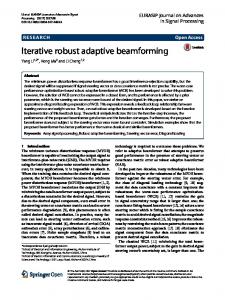
Figure 1: Comparison of the normalized beam patterns in Example 1 with SNR = 0 dB and 𝐾 = 60.
Example 2 (mismatch due to ASV random error). In this simulation example, the ASV of DS is assumed to be randomly distributed in an uncertainty set, which can be modeled as a (𝜃𝑠 ) = a (𝜃𝑠 ) + e,
(23)
where a(𝜃𝑠 ) represents the nominal SV corresponding to the direction 𝜃𝑠 and e is the random error vector, which is drawn in each simulation run independently from an uncertainty set as follows [12]: which means the mismatch changes from run to run but keeps fixed from snapshot to snapshot. The array normalized beam patterns for the beamformers in a single simulation run where SNR = 0 dB and 𝐾 = 60 are displayed in Figure 1. It can be seen that, in the presence of pointing error, the proposed beamformer and ESB beamformer are able to point the main lobe to the actual direction, while the LSMI beamformer and worst-case-based beamformer cannot. Furthermore, the proposed beamformer has lower side lobes and deeper nulls at the directions of interferences, which make the proposed beamformer suppress the noise and interferences effectively. Considering the influence of random look direction error on array output SINR, the performance curves versus the input SNR and the number of snapshots are drawn in Figures 2(a) and 2(b), respectively. The number of snapshots is fixed to be 𝐾 = 60 and the INR is kept at 30 dB in Figure 2(a), while a fixed SNR for the DS at 10 dB and a fixed INR at 30 dB are considered in Figure 2(b). From the results shown in Figure 2, it can be found that the output SINR of the proposed algorithm is closer to the optimal SINR in a large range of SNR from −10 to 50 dB and for all values of number of snapshots from 10 to 100, which illustrates its high dynamic range. That means the proposed algorithm outperforms the other tested beamformers in the scenario where only signal direction error exists. The SINR performance versus the pointing error is also investigated, and the results are shown in Figure 3 with fixed SNR and INR at 10 dB and 30 dB, respectively. It can be see that the proposed beamformer effectively deals with a wide range of pointing errors and achieves the best performance among the tested beamformers even when the pointing error is as large as ±4∘ .
e=
𝜀 [𝑒𝑗𝜙0 , 𝑒𝑗𝜙1 , . . . , 𝑒𝑗𝜙𝑀−1 ] , √𝑀
(24)
where 𝜀 and 𝜙𝑚 are uniformly distributed in the intervals [0, √3] and [0, 2𝜋], respectively. Figures 4(a) and 4(b) correspond to the performance of the investigated methods versus the input SNR and the number of snapshots. It can be seen from the figures that the proposed beamformer and the reconstruction-based beamformer outperform the other tested beamformers. Table 1 shows the deviations from the optimal SINR for the beamformers at SNR = 0 dB and SNR = 30 dB, respectively. The performance improvement is a direct result of the ASV estimation and DS elimination, especially at high SNR values. Furthermore, the proposed algorithm performs almost as well as the reconstruction-based beamformer for the output SINR but enjoys a faster convergence rate because of the lower computational cost without complex integral computation. Since the ASV mismatch is comprehensive and arbitrarytype, the proposed beamformer is proved to be effective against the random error of ASV. Example 3 (mismatch due to incoherent local scattering). In this example, it is assumed that the desired signal has a timevarying ASV which can be modeled as [11] 4
a (𝜃𝑠 ; 𝑘) = 𝑢0 (𝑘) a (𝜃𝑠 ) + ∑ 𝑢𝑝 (𝑘) a (𝜃𝑝 ) ,
(25)
𝑝=1
where a (𝜃𝑝 ), without loss of generality, 𝑝 = 1, 2, 3, 4, denotes the incoherently scattered signal paths. Assume that the
International Journal of Antennas and Propagation 70
25
60
20
50
15
40
Output SINR (dB)
Output SINR (dB)
6
30 20 10
10 5 0
−5 −10
0
−15
−10
−20
−20 −10
0
10
20
30
40
50
SNR (dB)
−25 10
20
30
40
50
60
70
80
90
100
Number of snapshots
Optimal Proposed beamformer LSMI beamformer Worst-case beamformer
ESB beamformer SQP beamformer Reconstruction-based beamformer Beamformer in [13]
(a)
Optimal Proposed beamformer LSMI beamformer Worst-case beamformer
ESB beamformer SQP beamformer Reconstruction-based beamformer Beamformer in [13]
(b)
Figure 2: Performance of the beamformers for the case of mismatch due to signal direction error. (a) Output SINR versus SNR for training data size of 𝐾 = 60 and INR = 30 dB. (b) Output SINR versus number of snapshots for fixed SNR = 10 dB and INR = 30 dB.
In this scenario, the signal covariance matrix Rs is no longer a rank-one matrix; thus the output SINR should be rewritten in a more general form [9]:
20
Output SINR (dB)
10 0
SINRopt =
−10
(26)
which is maximized by [9]
−20
−1 Rs } , wopt = 𝑃 {Ri+n
−30 −40 −50 −4
w𝐻Rs w , w𝐻Ri+n w
−3
−2
0 1 −1 Pointing error (∘ )
Optimal Proposed beamformer LSMI beamformer Worst-case beamformer
2
3
4
ESB beamformer SQP beamformer Reconstruction-based beamformer Beamformer in [13]
Figure 3: Output SINR versus pointing error for training data size of 𝐾 = 60 and SNR = 10 dB and INR = 30 dB.
directions 𝜃𝑝 are randomly distributed in a Gaussian distribution with mean 𝜃𝑠 and standard deviation 2∘ ; 𝑢0 (𝑘) and 𝑢𝑝 (𝑘) are independently and identically distributed complex Gaussian random variables drawn from 𝑁(0, 1) which change from snapshot to snapshot.
(27)
where 𝑃{⋅} denotes the same operation as in (11). Figures 5(a) and 5(b) show the performance curves versus the input SNR and the number of snapshots. It can be seen from the figures that the proposed beamformer presents an effective performance when handling incoherent local scattering. Similar to Example 2, in detail, there is about 0.8 dB performance loss for the proposed algorithm comparing to the reconstructionbased beamformer. The main reason is that the DS may leak into the complement sector Θ due to the incoherent local scattering, which affects the accuracy of the ASV estimation. Example 4 (impacts of some factors on performance). The main purpose of this example is to study the impacts of some factors on performance. 𝜉 and Δ are two main factors in the proposed algorithm. The former affects the accuracy of the construction of subspace in which the actual ASV a(𝜃𝑠 ) lies, and the latter decides the choice of taper matrix which plays a key role in the reconstruction of IPN covariance matrix. For the purpose of studying the impacts of the two factors, the model of the mismatch is set to be the same as the first example. The number of snapshots is fixed to be 𝐾 = 50;
International Journal of Antennas and Propagation
7 25
70
20
60
15
50
10
Output SINR (dB)
Output SINR (dB)
80
40 30 20 10
5 0
−5
0
−10
−10
−15
−20 −10
0
10
20
30
40
−20 10
50
20
30
Optimal Proposed beamformer LSMI beamformer Worst-case beamformer
40
50
60
70
80
90
100
Number of snapshots
SNR (dB)
Optimal Proposed beamformer LSMI beamformer Worst-case beamformer
ESB beamformer SQP beamformer Reconstruction-based beamformer Beamformer in [13]
(a)
ESB beamformer SQP beamformer Reconstruction-based beamformer Beamformer in [13]
(b)
Figure 4: Performance of the beamformers for the case of ASV random error. (a) Output SINR versus SNR for training data size of 𝐾 = 60 and INR = 30 dB. (b) Output SINR versus number of snapshots for fixed SNR = 10 dB and INR = 30 dB. 80
25
70
20 15
50
Output SINR (dB)
Output SINR (dB)
60
40 30 20 10
5 0
−5
0
−10
−10
−20 −10
10
0
10
20
30
40
50
SNR (dB) Optimal Proposed beamformer LSMI beamformer Worst-case beamformer
−15 10
20
30
40
50
60
70
80
90
100
Number of snapshots ESB beamformer SQP beamformer Reconstruction-based beamformer Beamformer in [13]
(a)
Optimal Proposed beamformer LSMI beamformer Worst-case beamformer
ESB beamformer SQP beamformer Reconstruction-based beamformer Beamformer in [13]
(b)
Figure 5: Performance of the beamformers for the case of incoherent local scattering. (a) Output SINR versus SNR for training data size of 𝐾 = 60 and INR = 30 dB. (b) Output SINR versus number of snapshots for fixed SNR = 10 dB and INR = 30 dB.
the INR and SNR are kept at 20 dB and 10 dB, respectively. The performances of the proposed algorithm versus 𝜉 and Δ are displayed in Figures 6(a) and 6(b), respectively. From Figure 6(a), it can be seen that the output SINR increases as 𝜉 gets larger, but the growth range is quite small. Considering
that the computational cost will not significantly increase as 𝜉 gets larger, setting 𝜉 = 0.95 in the proposed algorithm is appropriate. Similarly, the result of the test of Δ is shown in Figure 6(b), in which the choice of Δ = 2 arcsin(2/𝑀) can be found near the peak of the performance curve. To ensure a
8
International Journal of Antennas and Propagation 25
21.08 21.06
24 23
21.02
Output SINR (dB)
Output SINR (dB)
21.04
21 20.98 20.96 20.94
22 21 20
20.92 19
20.9 20.88
0
0.1
0.2
0.3
0.4
0.5
0.6
0.7
0.8
0.9
1
18
0
0.5
1
1.5
2
2.5
Proposed beamformer
(a)
3
3.5
4
4.5
5
Δ
𝜉 Optimal Proposed beamformer
(b)
Figure 6: Performance of the beamformers for the case of mismatch due to signal direction error. (a) Output SINR versus 𝜉. (b) Output SINR versus Δ for training data size of 𝐾 = 50 and INR = 20 dB and SNR = 10 dB.
satisfying output performance, Δ can be decided by a test for a typical array before the algorithm operates. The procedure is offline and will not dramatically increase the system cost.
5. Conclusion In this paper, a novel low-complexity RAB method is proposed which is easier to realize in practical situations and more robust to the look direction mismatch than other existing algorithms. The ASV is estimated by a closedform formula so as to avoid utilizing the optimization software, and the IPN covariance matrix is reconstructed by a sampling progress. The proposed beamformer only requires prior knowledge of the antenna geometry and the angular sector in which the ASV is located. Simulation results have demonstrated that the proposed beamformer can achieve superior performance over the existing state of the art RAB methods. To simplify the illustration, the influence of the element pattern, the polarization, and the mutual coupling is not considered in this paper. However, these elements will be investigated in the future study.
Competing Interests The authors declare that they have no competing interests.
References [1] H. L. Van Trees, Optimum Array Processing, John Wiley & Sons, Hoboken, NJ, USA, 2002. [2] W. Liu and S. Weiss, Wideband Beamforming: Concepts and Techniques, John Wiley & Sons, Chichester, UK, 2010.
[3] H. Singh and R. M. Jha, “Trends in adaptive array processing,” International Journal of Antennas and Propagation, vol. 2012, Article ID 361768, 20 pages, 2012. [4] U. Nickel, “Array processing for radar: achievements and challenges,” International Journal of Antennas and Propagation, vol. 2013, Article ID 261230, 21 pages, 2013. [5] J. Capon, “High-resolution frequency-wavenumber spectrum analysis,” Proceedings of the IEEE, vol. 57, no. 8, pp. 1408–1418, 1969. [6] S. A. Vorobyov, “Principles of minimum variance robust adaptive beamforming design,” Signal Processing, vol. 93, no. 12, pp. 3264–3277, 2013. [7] L. Du, J. Li, and P. Stoica, “Fully automatic computation of diagonal loading levels for robust adaptive beamforming,” IEEE Transactions on Aerospace and Electronic Systems, vol. 46, no. 1, pp. 449–458, 2010. [8] L. Chang and C.-C. Yeh, “Performance of DMI and eigenspacebased beamformers,” IEEE Transactions on Antennas and Propagation, vol. 40, no. 11, pp. 1336–1348, 1992. [9] S. A. Vorobyov, A. B. Gershman, and Z.-Q. Luo, “Robust adaptive beamforming using worst-case performance optimization: a solution to the signal mismatch problem,” IEEE Transactions on Signal Processing, vol. 51, no. 2, pp. 313–324, 2003. [10] H. Li, K. Wang, C. Wang, Y. He, and X. Zhu, “Robust adaptive beamforming based on worst-case and norm constraint,” International Journal of Antennas & Propagation, vol. 2015, Article ID 765385, 7 pages, 2015. [11] Y. Gu and A. Leshem, “Robust adaptive beamforming based on interference covariance matrix reconstruction and steering vector estimation,” IEEE Transactions on Signal Processing, vol. 60, no. 7, pp. 3881–3885, 2012. [12] L. Huang, J. Zhang, X. Xu, and Z. Ye, “Robust adaptive beamforming with a novel interference-plus-noise covariance matrix reconstruction method,” IEEE Transactions on Signal Processing, vol. 63, no. 7, pp. 1643–1650, 2015.
International Journal of Antennas and Propagation [13] H. Ruan and R. C. De Lamare, “Robust adaptive beamforming using a low-complexity shrinkage-based mismatch estimation algorithm,” IEEE Signal Processing Letters, vol. 21, no. 1, pp. 60– 64, 2014. [14] Z. Zhang, W. Liu, W. Leng, A. Wang, and H. Shi, “Interferenceplus-noise covariance matrix reconstruction via spatial power spectrum sampling for robust adaptive beamforming,” IEEE Signal Processing Letters, vol. 23, no. 1, pp. 121–125, 2016. [15] J. R. Guerci, “Theory and application of covariance matrix tapers for robust adaptive beamforming,” IEEE Transactions on Signal Processing, vol. 47, no. 4, pp. 977–985, 1999. [16] A. Khabbazibasmenj, S. A. Vorobyov, and A. Hassanien, “Robust adaptive beamforming based on steering vector estimation with as little as possible prior information,” IEEE Transactions on Signal Processing, vol. 60, no. 6, pp. 2974–2987, 2012. [17] F. Shen, F. Chen, and J. Song, “Robust adaptive beamforming based on steering vector estimation and covariance matrix reconstruction,” IEEE Communications Letters, vol. 19, no. 9, pp. 1636–1639, 2015. [18] A. Hassanien, S. A. Vorobyov, and K. M. Wong, “Robust adaptive beamforming using sequential quadratic programming: an iterative solution to the mismatch problem,” IEEE Signal Processing Letters, vol. 15, pp. 733–736, 2008. [19] J. Zhuang and A. Manikas, “Interference cancellation beamforming robust to pointing errors,” IET Signal Processing, vol. 7, no. 2, pp. 120–127, 2013. [20] A. Elnashar, S. M. Elnoubi, and H. A. El-Mikati, “Further study on robust adaptive beamforming with optimum diagonal loading,” IEEE Transactions on Antennas and Propagation, vol. 54, no. 12, pp. 3647–3658, 2006.
9
International Journal of
Rotating Machinery
Engineering Journal of
Hindawi Publishing Corporation http://www.hindawi.com
Volume 2014
The Scientific World Journal Hindawi Publishing Corporation http://www.hindawi.com
Volume 2014
International Journal of
Distributed Sensor Networks
Journal of
Sensors Hindawi Publishing Corporation http://www.hindawi.com
Volume 2014
Hindawi Publishing Corporation http://www.hindawi.com
Volume 2014
Hindawi Publishing Corporation http://www.hindawi.com
Volume 2014
Journal of
Control Science and Engineering
Advances in
Civil Engineering Hindawi Publishing Corporation http://www.hindawi.com
Hindawi Publishing Corporation http://www.hindawi.com
Volume 2014
Volume 2014
Submit your manuscripts at http://www.hindawi.com Journal of
Journal of
Electrical and Computer Engineering
Robotics Hindawi Publishing Corporation http://www.hindawi.com
Hindawi Publishing Corporation http://www.hindawi.com
Volume 2014
Volume 2014
VLSI Design Advances in OptoElectronics
International Journal of
Navigation and Observation Hindawi Publishing Corporation http://www.hindawi.com
Volume 2014
Hindawi Publishing Corporation http://www.hindawi.com
Hindawi Publishing Corporation http://www.hindawi.com
Chemical Engineering Hindawi Publishing Corporation http://www.hindawi.com
Volume 2014
Volume 2014
Active and Passive Electronic Components
Antennas and Propagation Hindawi Publishing Corporation http://www.hindawi.com
Aerospace Engineering
Hindawi Publishing Corporation http://www.hindawi.com
Volume 2014
Hindawi Publishing Corporation http://www.hindawi.com
Volume 2014
Volume 2014
International Journal of
International Journal of
International Journal of
Modelling & Simulation in Engineering
Volume 2014
Hindawi Publishing Corporation http://www.hindawi.com
Volume 2014
Shock and Vibration Hindawi Publishing Corporation http://www.hindawi.com
Volume 2014
Advances in
Acoustics and Vibration Hindawi Publishing Corporation http://www.hindawi.com
Volume 2014