Robust Instance Recognition in Presence of Occlusion and Clutter

Robust Instance Recognition in Presence of Occlusion and Clutter Ujwal Bonde, Vijay Badrinarayanan, Roberto Cipolla University of Cambridge

Abstract. We present a robust learning based instance recognition framework from single view point clouds. Our framework is able to handle real-world instance recognition challenges, i.e, clutter, similar looking distractors and occlusion. Recent algorithms have separately tried to address the problem of clutter [9] and occlusion [16] but fail when these challenges are combined. In comparison we handle all challenges within a single framework. Our framework uses a soft label Random Forest [5] to learn discriminative shape features of an object and use them to classify both its location and pose. We propose a novel iterative training scheme for forests which maximizes the margin between classes to improve recognition accuracy, as compared to a conventional training procedure. The learnt forest outperforms template matching, DPM [7] in presence of similar looking distractors. Using occlusion information, computed from the depth data, the forest learns to emphasize the shape features from the visible regions thus making it robust to occlusion. We benchmark our system with the state-of-the-art recognition systems [9, 7] in challenging scenes drawn from the largest publicly available dataset. To complement the lack of occlusion tests in this dataset, we introduce our Desk3D dataset and demonstrate that our algorithm outperforms other methods in all settings.

1

Introduction

A key limitation of supervised learning for object recognition is the need for large amounts of labelled training data so as to make it applicable to real world systems. One possible solution to address this limitation is to generate synthetic training data which closely resembles real world scenarios [21]. Object instance recognition is one such potential application where realistic training data can be easily synthesized using 3D object scans (using a Kinect sensor or dense reconstruction [17]) or which are available in large repositories such as the Google 3D warehouse [8]. Instance recognition in the presence of clutter and occlusion has several important applications, particularly in robotics and augmented reality. Recent methods [9, 10, 16, 6] have begun to exploit the availability of cheap depth sensors to achieve success in instance recognition. Unlike earlier methods that relied on clean laser scanned data [14], these devices have encouraged research into the use of cheap depth data for real-time applications. However, these sensors are relatively noisy and contain missing depth values, thus making it difficult

2

U. Bonde, V. Badrinarayanan, R. Cipolla

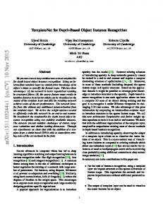
Fig. 1. Sample results of our instance recognition method which uses only point clouds as input. Meshed scenes from our Desk3D dataset with results of detection and pose classification on five object instances. Note meshed scenes are shown only for better visualization. Best viewed in color. See supplementary for videos.

to extract reliable object shape information. Recent development in 3D reconstruction [17] has made reliable shape information available in real time. In this work, we explore its use as an input for instance recognition (Fig. 1). However, to avoid being overly dependent on any particular reconstruction algorithm or sensor we use point clouds as input for recognition. Object shape, unlike color, is invariant to changes in illumination or texture. The availability of cheap and real-time 3D data encourages the use of shape as a cue for recognition, particularly when color and texture cues are unreliable. An important example is in robotics, where the objects of interest can be textureless and often greased or discoloured. However, results from the state-of-the-art algorithm (LineMod) indicate that color is the dominant cue [9] and it outperforms depth cues in the majority of instances that were tested. In LineMod, surface normals were sampled densely over each 2.5D object template and these were used as depth cues for template matching. We believe this approach has not fully utilized the potential of depth data, especially the information present in the internal and external edges (contours) of the object. Moreover, a lack of discriminative selection of shape features in their approach degrades performance under presence of clutter and similar looking distractors. In contrast, given a 3D point-cloud model of an object, we encode its 3D shape using a discriminative set of edgelet/normal features learnt using a soft-label Random forest (slRF) [5]. Popular approaches to occlusion based recognition mainly rely on a partsbased strategy where the object is divided into smaller parts which vote for the presence of an object [14]. However as demonstrated in Sec. 4 most current depth based recognition systems suffer when the size of the object decreases. For this reason we explore the use of depth based occlusion cues similar to [16]. However compared to their work which uses multiple views along with its depth data, we

Robust Instance Recognition in Presence of Occlusion and Clutter

3

only require the occlusion cues from a single view point cloud data. Moreover unlike their multi-staged approach that uses heuristic weighting functions our framework uses a single-stage slRF which learns to emphasize shape cues from visible region. In recent years, several real-world RGB-D datasets have been published for object recognition [15, 16, 22]. The test scenes in these datasets either have a relatively clean background with not enough pose variations [16, 22] or have no occlusion [15]. In the absence of such a dataset we create a new challenging dataset containing clutter as well as occlusion. We term this ground-truthed database as Desk3D. In the Desk3D dataset, each scene point-cloud is obtained by integrating few frames of depth data from a Kinect sensor to aid in better extraction of edge features. Moreover, to better demonstrate the benefits of our learning based recognition scheme, we also use the publicly available dataset (ACCV3D) [10] which has the largest number of test pose variations in the presence of heavy clutter with no occlusion. We benchmark our algorithm by extensive evaluation on Desk3D as well as on ACCV3D and show that our learning based method clearly outperforms the state-of-the-art recognition algorithms. To summarize, our contributions are as follows: 1. We jointly address multiple instance recognition challenges of occlusion, clutter and similar looking distractors within a single learning based framework. 2. We introduce the challenging Desk3D dataset containing multiple clutter and occlusion scenarios to benchmark instance recognition methods.

2

Literature Review

A large portion of existing literature in instance recognition is dedicated to building descriptors to improve recognition [23, 2]. In this work we use simple edge/normal orientation features and focus on achieving robust recognition in presence of clutter, similar looking distractors and occlusion. However these simple features can be replaced by more complex features that exist in literature. Hinterstoisser et al. [9] use simple orientations features densely sampled to build robustness which they call the Dominant Orientation Templates (DOT). Using thousands of such templates for different viewpoints along with multimodal signals (RGB+Depth) they achieve robustness to random clutter. RiosCabrera et al. [20] extend this work by discriminatively learning both the sampled features as well as the templates. Using a boosted classifier they are able to perform real time recognition on 10-15 objects. However as they still rely on 2D template matching its not clear how this work could be extended to handle occlusions as seen in the real world. In contrast our random forest framework exploits the depth ordering in single view for robustness to occlusion. There has been a recent surge of interest in occlusion reasoning for object recognition [11, 27, 25]. These methods have primarily focused on jointly determining the occlusion and object location in single view RGB images. In this work, we are primarily interested in improving the robustness in presence of occlusion by utilizing the information obtained from single view point clouds. Our

4

U. Bonde, V. Badrinarayanan, R. Cipolla 3D Scan

Quantized Pose Classes

Quantize and Voxelize Feature Orientations

Simulate 2.5D Views

Compute Label Vector 0.04 0.35 0.17

Robust Multi-Class slRF Training Q1

0.13 0

Normalized distance from quantized pose class

Fg/ Bg

Compute Dominant Orientations

Compute Occlusion States

Q2 Q3

Car

Not Car

Fig. 2. Our training pipeline. Given a 3D object scan (point cloud) we simulate several thousand 2.5D object views, extract features for each view at various voxel offsets and assign them soft labels using the quantized pose classes. These features and soft labels are used to train a multi-class soft label Random Forest (slRF) [5] in a novel iterative manner to jointly classify location and pose of an object.

work is similar to [16] wherein they use multi-view RGB and depth images to compute occlusion information. Using multiple stages of reasoning along with a DPM [7] they achieve robustness to occlusion. In contrast we use a single-stage slRF which learns to emphasize shape cues from visible regions. Deformable parts model have been successfully used for object category recognition [7]. Recently this has also been extended to object instance recognition in RGB [26]. However DPM’s natural ability to exploit the similarity that exist within a category makes it unsuitable for detection in presence of similar looking distractors. On the other hand our slRF learns the most discriminative features for a given instance and hence is better able to deal with similar objects.

3

Learning Approach

An overview of our learning system is shown in Fig. 2. The input is a point cloud which is obtained from raw depth frames using Kinect or by integrating a few frames (typically 5-10 using Kinect Fusion [19]). The advantage of the latter approach is that it reduces noise and missing data from the sensor with minimal blurring of details. This makes it a stable input to estimate edges on the resulting point clouds. An advantage of working with point clouds is that the physical dimension of the scene does not change with the distance it is captured from. This eliminates the need to search over different object sizes for recognition. We first perform edgelet detection on point clouds as described below. 3.1

Edgelet Detection

Using the multi-scale method of Bonde et al. [3] we calculate the two principal curvatures λ1 , λ2 for every point on the point cloud. We only consider the magnitude of the principal curvatures. In a point cloud, edges are regions where one of the principal curvatures is considerably larger than the other, i.e a ridge

Robust Instance Recognition in Presence of Occlusion and Clutter

5

or a valley. For this reason, we consider the ratio of the principal curvatures r = λλ21 , where λ1 ≥ λ2 . Since the point cloud is obtained from a few consecutive frames (or a single frame) we can consider it to be from a single-view. We convert it into a curvature map, where each pixel stores the ratio r. Using hysteresis thresholding [18] we detect connected regions of high r. We perform non-maximal suppression on these regions to get the internal edges. Contours or external edges are regions where depth discontinuities are large. To detect these view dependent edges, we convert the single-view point cloud into a range image. Again, using hysteresis thresholding we detect regions of high depth discontinuities to obtain the external edges. These regions/edges are back projected onto the point cloud to get all the edgelet points (see Fig. 4). Finally, using local RANSAC line fitting we detect the orientation for each edgelet point. The orientations are quantized into 8 bins similar to [9] (to avoid ambiguity, we only consider camera facing orientations). 3.2

Encoding Occlusion aware Features

We use a full 360 degree scan of the object for training. This scan is used to simulate different 2.5D views of the object. In each simulated view, edgelets are detected as described in Sec. 3.1. These edgelet points are quantized into a fixed voxel grid of size w × h × d (typical values are 6 − 8). The dominant orientation of a voxel (v) is obtained by histogramming the orientation of all edgelet points within it and choosing the bin with maximum value. However, voxels containing corners or high curvature edges can have multiple dominant orientations. Therefore, at each voxel we also select all orientations whose histogram value is greater than one third the maximum value as dominant orientations. To achieve robustness to noise, we only consider those orientations whose histogram value is greater than a threshold (typically 10−30). The feature vector for each voxel v is thus a vector xv with eight elements and an element value is equal to 1 if the corresponding orientation is dominant. Given the point cloud for the j th view we simulate an occluder in front of the object. Inspired by [11] we use a box world model for the occluder which are rectangular screens placed in front of the objects. The dimension of the screen have a truncated Gaussian distribution centered on 1/3rd the dimensions of the simulated point cloud. As most natural occluders are resting on ground we simulate the occluder to start from the ground plane and not hanging in mid-air. Given the resulting point cloud we remove the occluded points from the simulated object. Using ray tracing (Fig 2) we assign an occlusion state Ov = 1 (or 0) for each of the visible voxels (or occluded) in the w × h × d voxel grid. Finallyfor all the occluded voxels we modify their feature vector xv = − 1 where, −1 is an eight element vector with all elements −1. The resulting feature vector encodes the three possible states: -1 for occluded voxel, 0 for visible but no dominant orientation and 1 for visible and dominant orientation. Finally, we concatenated the vectors for all voxel in the j th view to get a feature vector xj of dimension w × h × d × 8.

6

3.3

U. Bonde, V. Badrinarayanan, R. Cipolla

Robust training of soft label Random Forest:

Soft Labelling: In order to assign labels for the simulated views, we first uniformly quantize the object viewpoints into 16 pose classes (2 along pitch, 2 along roll and 4 along yaw). As a simulated pose could be between two quantized pose classes it is assigned a soft-label with respect to each pose class. This helps to better explain simulated poses that are not close to any single pose class (see Sec. 3.5). Soft labels for each simulated pose are assigned based on the deviation of its canonical rotational matrix to the identity matrix [12]. For example, if Rji represents the canonical rotation matrix to take the j th simulated view to the ith quantized pose, then its distance is given by: dij = kI − Rji kF , where I is a 3 × 3 identity matrix and k.kF is the Frobenius norm. The soft labels are then given by: 2

lji = exp(−dij ), i ∈ {1, ..., 16} .

(1)

The final label vector for a simulated pose is normalized as i=1:16 lji = 1. We also add an additional label (16+1) to indicate foreground (fg) or background (bg) class. This is set to 0 for the simulated views (fg) and 1 for the bg examples (all the other 16 elements in the label vector are set to 0 in this case). We generate about 27000 such simulated views w/o occlusion and a similar number with occlusion spanning all the views of the object. For robustness, we augment the fg training set with a shifted version (2 voxels along all axes) of the simulated views. To improve localization, we augment the bg training set with a large shifted version (8 voxels) of the simulated views. Given the complete training data X = {xj , lj } a conventional 16+1 multi-class slRF is trained using the whole data. Similar to a multi-class RF, slRF computes a histogram of class membership at each node by element wise addition of the soft labels across all training examples falling into it. The split functions (features) query for occluded/presence or absence of a dominant orientation within a voxel. An information entropy measure [5] is used to evaluate the split function. We refer the reader to [5] for a detailed description of conventional slRF training. Each leaf node (Lf ) in the trained slRF stores the foreground probability (pf g ) as the ratio of positive (fg)  to negative (bg) samples  as well as the P

pose class probabilities for fg samples

pips =

i j∈Lf lj

P

P

j∈Lf

i i∈[1,16] lj

P

. Note here that

all the simulated views are considered as positive or fg samples irrespective of their pose. This is because the label assignment (Eq. 1) distributes the fg probability over all 16 pose classes. During testing fg and pose class probabilities are summed over 100 trees to get pf g , pbg for the forest. Occlusion Queries: Given the tertiary nature of our feature vector xj ∈ {−1, 0, 1} two types of split questions exist. One which queries (> −1) for visible versus occluded voxel while the other queries (> 0) for a dominant orientation in a visible voxel. During the training of our slRF, split questions in the topmost nodes (≈ 5 − 10) are restricted to only the second type of query. This is in accordance with the intuition that the decision for the presence of an object can be made from the features (dominant orientations) present in the visible regions

Robust Instance Recognition in Presence of Occlusion and Clutter 3

Foreground Background

b)

2 1.5 1 0.5 0 0

3

Foreground Background

c)

2.5

# of Samples

# of Samples

2.5

2 1.5 1 0.5

0.2

0.4

0.6

0.8

Foreground Probability

1

0 0

x 10

3

Foreground Background

d)

2.5 2 1.5 1 0.5

0.2

0.4

0.6

0.8

Foreground Probability

1

0 0

7

5

5

# of Samples

3

a)

5

x 10

x 10

Foreground Background

2.5

# of Samples

5

x 10

2 1.5 1 0.5

0.2

0.4

0.6

0.8

Foreground Probability

1

0 0

0.2 0.4 0.6 0.8 Foreground Probability

1

Fig. 3. (a) Foreground (fg) probability of training samples after conventional training of the slRF. No clear margin exists between the two classes. (b,c,d) show the fg probability over increasing number of iterations using our robust iterative training scheme (Alg. 1). A clear margin is visible between the class samples as the iterations progress.

and not based on the visibility/occlusion of a voxels. We remove this restriction for the bottom layers which allows the slRF to branch out based on the visibility of voxels and emphasize questions from visible regions. Maximizing the Margin between Classes: Fig. 3(a) shows the pf g predicted by the conventional slRF on the training data X for a sample class. We can observe that a subset of the two classes overlap and there does not exist a clear margin between the fg and bg samples. For robust recognition, we would ideally like to have a clear margin that would allow us to deal with sensor noise and also define a detection threshold. To this end, we propose an novel iterative training scheme which automatically mines these difficult examples lying in the overlapping parts and uses these to increase the margin between the two classes. We start by randomly selecting a subset of the training data Xs ⊂ X such that |Xs |  |X|. We then train a multi-class slRF with this subset |Xs | and calculate the leaf node distributions using the entire training corpus X. From the computed pf g we then select borderline positives (fg examples with low pf g ) and borderline negatives (bg examples with high pf g ) and augment |Xs | with these examples. However, for the classifier to learn to distinguish between borderline positive and similar or confusing negative examples, and vice versa, we also need to add these confusing examples to the training set. To mine the confusing negative examples we search for those negative examples that share the maximal number of leaf nodes with the borderline positive examples (and vice versa). Further, since our goal is to jointly predict both the location and pose, we follow a similar strategy for pose. After each iteration, we rank the accuracy of pose classification for each foreground sample as: djL = (ljc − ˆljc )/ljc , where c = arg maxi lji and ˆlj is the predicted class label vector. We then augment the training set with positive example having the largest dL . Figs. 3 (b,c,d) show the fg probability margin increasing between fg and bg samples over iterations. Unlike most bootstrapping approaches, we start with a small training set for computational efficiency and low memory consumption. In our work, |Xs | ≈ |X|/20. After each iteration we add a total of |X|/20 examples. We continue the process until the fg probability of all positive samples is greater than the fg probability of all negative samples. Usually this take 5-10 iterations. Our method shares some similarity to the work of [24], but they do not mine the confusing/similar examples which is crucial to establish the margin. We em-

8

U. Bonde, V. Badrinarayanan, R. Cipolla

Algorithm 1: Proposed iterative training scheme for slRF. Input: Training set X = {xj , lj } Output: Learnt slRF classifier 1. Randomly select a subset: Xs ⊂ X such that |Xs | = |X|/20. 2. Train slRF with Xs and compute pf g for all X (see Sec. 3.3). 3. Augment Xs with borderline positive (low pf g ) and borderline negative (high pf g ). 4. Locate and augment Xs with confusing negative/ positive samples (see Sec. 3.3). 5. Compute pose class prediction accuracies dL for all positive samples (see Sec. 3.3) and augment Xs with positive examples having high dL . 6. Repeat steps 2 to 5 till pf g for all positive data is greater than pf g for all negative data.

phasize that this difference is crucial to achieve robustness Fig. 6(c) shows the performance improvement by mining these confusing examples. Alg. 1 summarizes the steps of our training scheme. 3.4

Addressing Challenges of Clutter and Occlusion

Robustness to Clutter: In Sec. 3.3 we described the our iterative algorithm which increases the margin between similar looking examples. This increases the robustness of our framework allowing it reliably recognize difficult poses even in the presence of clutter (Fig. 6). Dealing with Similar Looking Distractors We set up an example case to understand how the slRF learns to discriminate between an object of interest and a similar looking distractor(s). We chose two car instances, a Mini and a Ferrari toy model (see Fig. 4). We select a quantized pose class and visualize the features (queries) learnt by their respective slRF by picking out all the training examples whose label vectors give this pose the maximum probability. We then pass these examples through the corresponding slRF. We select and plot the top few features that were repeatedly used as a node split feature (or queries) by the respective slRF (see Fig. 4). Each bold arrow in the figure represents an edgelet orientation query (feature). A pair or triplet of arrows correspond to multiple queries within a voxel. Note that different colors are used to represent the orientation queries and the encircled edgelets of the same color are those which responded positively to them. For the Mini, the queries capture the edgelets forming a corner of its windshield. For the Ferrari, the windshield and roof are smooth and hence no edgelets are detected at the windshield. On the other hand, the Ferrari’s curved roof is a distinct feature which is captured by its slRF. These queries fail to find enough response on the Mini. Note that the slRF learns to query shape cues apart from simple corners. Occlusion Training: To understand how the slRF uses the occlusion information we test two sample scenarios for the toy mini each having the same pose. For the first scenario, we generate examples wherein the front portion of the mini is occluded, while for the second scenario we occlude the middle portion. We then select the most frequently asked questions for both scenarios and only plot those questions that do not overlap in both scenarios. Fig. 4 (right top) shows the frequently asked questions for front occlusion which are absent in the

Robust Instance Recognition in Presence of Occlusion and Clutter Learnt Queries for Mini

Low response on Ferrari for learnt Mini Queries

Low response on Mini for learnt Ferrari Queries

Learnt Queries for Ferrari

9

Questions for Front Occlusion

Questions for Middle Occlusion

Fig. 4. Edgelet maps and some learnt features (queries) for a quantized pose class of the Ferrari and Mini. Left pane shows that when the learnt dominant orientation queries for the Mini (windshield) are projected onto the Ferrari they fail to find sufficient response. Similarly, Middle pane shows the learnt queries for the Ferrari (curved roof) fail to find sufficient response on the Mini. Note that the queries correspond to more than just corners and often capture intuitive shape features on the objects (see Sec. 3.4). Right pane shows the difference in the learnt dominant orientations when front/middle portion of Mini are occluded. Based on the occlusion information the slRF learns to emphasize questions from visible regions.

second scenario. We observe that these questions shift to the middle/back (visible) portion of the mini. We also observe questions on the top portion of the front car. This is because of our assumption on the occluder model (Gaussian prior with the occluders resting on ground) which assigns a greater probability of the top portion been visible. Fig. 4 (right bottom) show the frequently asked questions for middle occlusion that are missing in the first scenario. A similar behavior is observed. This indicates that the slRF is using the occlusion questions to emphasize the visible portions and queries these regions to better deal with occlusion. Note that as compared to [16] who use a heuristic weighting our method automatically learns this from the occlusion queries. 3.5

Testing

We test our system on our Desk3D dataset as well as the publicly available ACCV3D dataset. For the Desk3D dataset, during testing, point clouds are obtained from the integration of a few Kinect frames (5) over a fixed region (1.25m × 1.25m × 1.25m). For the ACCV3D dataset, point clouds are obtained from individual depth frames to allow a fair comparison to other methods. This is followed by edgelet detection on the point cloud. The resulting edgelet points are voxelized into a 128 × 128 × 128 grid. We then compute shape features and occlusion states for these voxels as in the training stage. A sliding cuboid search is performed on the voxel grid. For each voxel location, the slRF is used to compute

U. Bonde, V. Badrinarayanan, R. Cipolla 1

1

b)

0.6

0.4

0.2

0 0

0.2

0.4

0.6

Recall

0.6

0.4

0.2

LineMod LineModSup S−Iterative(Normal) 0.8

1

c)

0.8

Precision

Precision

0.8

Precision

a)

0 0

0.4

0.6

Recall

1

1

0.8

0.8

0.8

1

d)

0.6

0.4

0.2

LineMod LineModSup S−Iterative(Normal) 0.2

Average for all Obj. Inst. in Desk3D

Average for all Obj. Inst. in Desk3D

Average for Small Obj. Inst.(ACCV3D)

Average for Large Obj. Inst.(ACCV3D)

Precision

10

0 0

LineModSupp S−Iterative(Normal) S−Iterative(Edge) S−Iterative(Edge+Occlusion) DPM 0.2

0.4

0.6

Recall

0.8

0.6

0.4

0.2

1

0 0

H−All(Edge) S−All(Edge) S−Iterative(Edge) 0.2

0.4

0.6

Recall

0.8

1

Fig. 5. Precision-Recall (PR) curves for joint pose+location. (a) and (b) PR curves for the ACCV3D dataset comparing LineMod with supervised removal of confusing templates (LineModSup) and w/o supervision, and our robust slRF (S-Iterative(Normals)). For fairness, we used surface normal features in our method as in LineMod. We clearly outperform LineMod and LineModSup on large objects. For small objects all methods do equally bad due to poor sensor resolution. (c) PR curves on non-occluded samples of Desk3D dataset for LineModSup, S-Iterative(Normals/Edge/Edge+Occlusion) and DPM. S-Iterative(Edge/Edge+Occlusion) outperform all other methods as they use both internal edge and contour cues for discrimination. DPM with HOG on depth images cannot not capture these details and performs poorly. (d) PR curves on Desk3D comparing hard (H-All(Edge)), soft label RF (S-All(Edge)) using conventional training. The use of soft-labels provides clear benefit over hard/scalar labels at high recall rates where several test examples which are not close to the quantized pose classes occur. Our robustly trained slRF (S-Iterative(Edge)) is more accurate as it learns a margin between classes.

the fg class and pose probabilities. We pick the voxel with the maximum pf g as the detected location and choose the pose class with the maximum pps . Note that we do not consider voxels close to the boundary of the grid. Also, we only consider voxel locations which have a sufficient number of edgelets within them.

4

Experiments and Results

We benchmark our system using the publicly available ACCV3D dataset [9] containing the largest number of test pose variation per object instance. Unlike other existing datasets [15, 4, 22] this dataset has high clutter and pose variations, thus closely approximating real world conditions. ACCV3D contains instances of 15 objects, each having over 1100 test frames (also see supplementary videos). For more extensive comparisons, we also tested on our Desk3D dataset. Desk3D contains multiple desktop test scenarios, where each test frame is obtained by integrating a few (5) frames from the Kinect sensor (see Fig. 4). In total there are over 850 test scenes containing six objects. The dataset also contains 450 test scenes with no objects to test the accuracy of the system. Scenario 1: Here we place two similar looking objects (Mini and Ferrari) along with similar looking distractors to confuse the recognition systems (see supplementary video). There are three test scenes wherein the objects are placed in different locations and poses. Each test scene/frame is recorded by smoothly moving the Kinect sensor over the scene. 110 test frames are automatically

Robust Instance Recognition in Presence of Occlusion and Clutter

11

Avg. for Obj. Inst. Mini 1

a)

b)

c) Precision

0.8

0.6

0.4

0.2

0 0

S−Iterative (confusing ex.)−L+P S−Iterative (confusing ex.)−L S−Iterative (w/o confusing ex.)−L+P S−Iterative (w/o confusing ex.)−L

0.2

0.4

0.6

Recall

0.8

Fig. 6. Precision-Recall curves (joint pose+location) for the Mini on (a) near-back poses; (b) near-front poses in Desk3D . (c) PR curves (both location and joint pose+location) comparing the performance by mining confusing examples(see Sec. 3.3). Our iteratively trained slRF maximizes the margin between fg and bg (Sec. 3.3) and thus shows a large improvement on difficult poses compared to conventional training.

ground truthed using a known pattern on the desk (see Fig. 1). Scenario 2: Here we test the performance of the algorithms in low clutter. We have five objects (Face, Kettle, Mini, Phone and Statue) of different 3D shape. We place the objects in clutter and record 60 − 90 frames for each object. Scenario 3: Here we test the performance of the recognition algorithms in significant clutter. We capture six test scenes with the same five objects. Each test scene has 400 − 500 frames containing multiple objects with different backgrounds/clutter and poses. Scenario 4: This scenario tests the performance of the recognition algorithms in occlusion and clutter. Current instance recognition datasets do not contain this challenge. We capture five test scenes similar to earlier scenario containing multiple objects with different backgrounds/clutter and poses. For the background (bg) class, we record three scenes without any of the objects. The first two bg scenes contain 100 test frames each and are used as bg data to train the slRF. The third scene with 489 test frames are used to determine the accuracy of the learnt classifier. We quantify the performance of our proposed learning based system with the state-of-the-art template matching method of LineMod [9] using the two datasets. We use the open source implementation of their code [1]. For a fair comparison, we use only the depth modality based recognition set up of their system. As LineMod treats RGB/Depth separately and combines their individual matching score at the last stage of the detection pipeline, removing the RGB modality does not affect the training or testing of their depth alone system. As in our method, we train their system using the simulated views generated for each object. These simulated views are projected at different depths to learn scale-invariance for LineMod. Finally, their online training is used to learn the object templates. Except for the face category and small objects, each object instance contained more than 3000 templates after training. We observed that some of these learnt templates were often confused with the background. For this reason, we add a supervised stage wherein we test their detector on the

1

12

U. Bonde, V. Badrinarayanan, R. Cipolla LineMod [9] Object Instance BenchVise Camera Can Driller Iron Lamp Phone Bowl Box Avg.(Large) Ape Duck Cat Cup Glue Holepunch Avg.(Small) Avg.(All)

L 82.88 67.94 67.98 92.85 53.99 89.81 53.02 75.43 96.49 75.60 28.32 50.80 60.81 30.48 14.67 28.21 33.88 59.58

L + P 74.57 57.70 56.44 69.11 44.01 75.39 48.27 14.92 55.31 55.08 17.96 37.72 49.19 18.55 07.70 22.31 23.91 43.28

LineMod [9] (Supervision) L L + P 83.79 75.23 77.19 68.94 83.70 69.57 94.70 81.82 83.51 75.43 92.91 80.93 77.72 70.47 98.11 19.22 63.37 27.69 84.00 63.26 22.98 07.36 30.94 19.46 63.10 53.69 72.98 27.90 21.48 10.25 36.54 31.20 41.34 24.98 66.93 47.94

L 87.98 58.20 94.73 91.16 84.98 99.59 88.09 98.54 95.21 88.62 25.32 50.00 50.55 73.55 62.70 73.00 55.85 75.58

Our Work L + P 86.50 53.37 86.42 87.63 70.75 98.04 87.69 30.66 63.53 73.64 19.90 39.70 44.27 42.82 42.54 70.01 43.10 61.43

Table 1. Comparison of our robust slRF with the state-of-the-art LineMod method on the ACCV3D dataset. We report both location only (L) and joint location and pose classification (L+P) results for both large and small objects. We outperform LineMod clearly with large objects and even with small objects, on an average, we perform better. Moreover, our overall pose classification is superior to that of LineMod. We see a large improvement on objects which have mainly smooth surfaces (can, holepunch, lamp, phone). For objects with high 3D detail (benchvise, driller, iron) all methods fare the same. Both systems are poor for very small objects (ape, cat, duck) as sensor resolution is low. Also, unlike LineMod, we currently do not adapt the size of voxels.

two background test scenes with 100 frames. We remove templates that give a positive detection with high score (80) more than 200 times, i.e on an average once per frame. This significantly improved their recognition performance. We also benchmark with DPM [7] which is widely considered as the state-of-theart for category recognition. We use DPM with HOG feature on the depth images as a baseline. For training we use the simulated views similar to those used for training our work and LineMod. We observe that DPM with HOG on depth images does a poor job in describing instances and hence does poorly. These results were in in accordance with earlier observations [13]. For this reason we only compare DPM on the Desk3D dataset. During testing, we consider localiza) of tion to be correct if the predicted center is within a fixed radius ( max(w,d,h) 3 the ground truth position. We consider pose classification to be correct if the predicted pose class (largest pose probability) or template is either the closest or second closest quantized pose to the ground truth. Analysis: Fig. 5(a) and (b) shows the average PR curves for large and small objects in ACCV3D and Table 1 shows the accuracies of the methods. Approximately, large (small) objects have their axis-aligned bounding box volume greater (lesser) than 1000cm3 . For a fair comparison, we used surface normal features as in LineMod. Overall we outperform LineMod (both with and w/o supervision) and a marked improvement is seen on pose classification. We have significant gains in performance on predominantly smooth objects (can, holepunch, lamp, phone) where dense feature sampling (LineMod) is confused by clutter. Both methods compare fairly on objects with more detail such as benchvise, driller, iron. Due to poor sensor resolution both methods perform poorly on small ob-

Robust Instance Recognition in Presence of Occlusion and Clutter 1

0.8

b)

0.6

0.4

0.2

0 0

LineModSupp S−Iterative(Normal) S−Iterative(Edge) S−Iterative(Edge+Occlusion) DPM 0.2

0.4

0.6

Recall

0.8

1

1

0.4

0 0

LineModSupp S−Iterative(Normal) S−Iterative(Edge) S−Iterative(Edge+Occlusion) DPM 0.2

0.4

0.6

Recall

0.8

1

1

d)

0.6

0.4

0.2

0 0

Average for Obj. Inst. with Occlusion

Test Scenario 3

0.8

c)

0.6

0.2

Average for Obj. Inst. in High Clutter

Test Scenario 2

0.8

Precision

Precision

a)

Average for Obj. Inst. in Low clutter

Test Scenario 1

Precision

1

LineModSupp S−Iterative(Normal) S−Iterative(Edge) S−Iterative(Edge+Occlusion) DPM 0.2

0.4

0.6

Recall

0.8

0.6

0.4

0.2

1

Test Scenario 4

0.8

Precision

Average for Obj. Inst. Mini & Ferrari

13

0 0

LineModSupp S−Iterative(Edge) S−Iterative(Edge+Occlusion) DPM 0.2

0.4

0.6

Recall

0.8

1

Fig. 7. PR curves for pose+location. (a) PR curves for test scenario 1 in Desk3D. Our discriminatively trained robust slRF (both SIterative(Normals/Edge/Edge+Occlusion)) clearly outperforms DPM and LineMod even with supervision (removal of confusing templates - LineModSup). (b) Even in low clutter scenario DPM with HOG features on depth images does poorly. All other methods perform reasonable well (c) In high clutter, our method clearly shows significant gain at high recall rates. LineMod’s dense feature sampling performs poorly on smooth objects.

jects (ape, cat, duck). Fig. 5(c) shows the average PR curves for Desk3D where our method outperforms LineMod even with supervision. Edgelets based slRF does better than surface normals based slRF as most objects in Desk3D (except Face, Kettle) have internal details which are better represented by edgelets. From Table 2 we can observe that iterative training with edgelet features performed best. A clear improvement is seen for similar looking ( Ferrari, Mini) where our approach learns their fine discriminative features (Fig. 7(a)). From Fig. 7(b) we can see that except DPM all the methods perform well under low clutter, but as the clutter is increased (Fig. 7(c)) we clearly outperform LineMod, DPM. As in ACCV3D, for predominantly smooth objects (Kettle, Phone) LineMod’s dense feature sampling performs poorly. For objects (Statue) which have high 3D detail the performance of all the methods are similar. For symmetrical objects (Face) pose classification suffers for all methods. From Table 3 and Fig. 7(d) we see that our occlusion based slRF outperforms all method. This is because it learns to emphasize questions from visible regions. In Fig. 5(d) we compare our slRF with conventional RF trained with hard/scalar labels. These scalar labels were assigned based on the pose class having the largest li (see Eq. 1). For pose classification, the conventional RF performs better at low recall rates as it does better than the slRF for test poses which are close to the quantized pose classes. However, for test poses which are further from the quantized pose classes, slRF fares better giving a higher precision at large recall rates. Fig. 5(d) also shows that our iteratively learnt slRF outperforms a conventional slRF. This is because our iterative strategy directs the slRF to concentrate harder on the difficult examples. To illustrate this, in Fig. 6(a) and (b) we show PR curves on two test scenes where the Mini is seen in nearback/front pose. Fig. 6(c) illustrates the advantage of mining confusing examples as proposed in Sec. 3.3 for the class Mini. Similar performance was seen on other classes as well.

14

U. Bonde, V. Badrinarayanan, R. Cipolla LineMod [9] Object Instance Face Kettle Ferrari Mini Phone Statue Average

L 88.66 76.19 24.37 26.22 53.55 90.15 59.86

L+P 45.57 38.80 12.61 12.27 43.85 83.27 39.39

LineMod [9] (Supervision) L L+P 91.55 66.60 83.95 60.49 75.63 47.90 68.76 55.09 89.77 79.03 91.64 84.76 83.95 65.64

DPM [7] (D-HoG) L L+P 73.40 44.74 65.32 53.34 52.14 32.41 53.26 30.64 57.43 64.32 74.50 70.29 64.34 49.29

H-All (Edges) L L+P 75.46 48.04 81.31 71.96 95.80 73.95 81.31 70.15 96.71 90.81 89.78 84.20 86.73 73.19

S-All (Edges) L L+P 84.12 49.90 82.19 73.02 98.32 74.79 84.80 73.22 97.05 91.68 89.22 85.50 89.29 74.68

S-Iterative (Edges) L L+P 87.01 52.99 87.83 78.48 98.32 77.31 87.03 76.71 96.53 90.99 91.45 86.25 91.36 77.12

S-Iterative (Occlusion) L L+P 74.02 44.33 89.77 79.19 96.64 65.55 87.87 79.78 96.71 91.16 91.75 86.80 89.46 74.47

Table 2. Comparison of our learning based system (for non-occluded scenes) under various training settings and features with the state-of-the-art instance recognition system (LineMod [9], DPM [7]) on the Desk3D dataset. We report location(L), joint location and pose classification (L+P) accuracies. H-All, S-All is conventional training with hard/soft labels respectively. S-Iterative is robust iterative training using soft labels. S-Iterative(Occlusion) uses the occlusion queries (see Sec. 3). Our system outperforms LineMod on 5/6 and DPM on all object instances. On an average, we outperform LineMod and DPM both with and w/o supervised removal of confusing templates (see Sec. 3.5). A marked improvement is seen in the discrimination between similar looking object instances (Ferrari, Mini). Object Instance Face Kettle Mini Phone Statue Average

LineMod [9] (Supervision) L L+P 73.21 26.29 12.83 8.38 37.42 16.67 20.13 12.46 06.67 02.05 30.15 13.17

DPM [7] (D-HoG) L L+P 44.00 08.86 47.82 35.32 40.50 20.39 37.19 23.21 32.97 30.31 40.50 23.72

S-Iterative (Edges) L+P 45.11 54.82 46.65 69.58 45.00 52.62

L 88.79 74.10 53.35 80.26 53.61 70.70

S-Iterative (Occlusion) L L+P 89.71 40.00 83.25 67.54 69.18 58.49 86.26 73.48 81.03 71.03 81.89 62.11

Table 3. Comparison of our learning based system with the state-of-the-art instance recognition system on occluded scenes in the Desk3D dataset. Our occlusion handling scheme is robust to occlusion and outperforms all methods by over 10%.

5

Conclusion

We presented a learning based approach for depth based object instance recognition from single view point clouds. Our goal was to robustly estimate both the location and pose of an object instance in scenes with clutter, simialr looking distractors and occlusion. We employ a multi-class soft-label Random Forest to perform joint classification of location and pose. We proposed a novel iterative margin-maximizing training scheme to boost the performance of the forest on classification of difficult poses in cluttered scenes. By exploiting the depth ordering in single view point cloud data our method performs robustly even in the presence of large occlusions. We evaluated the performance of our algorithm on the largest publicly available dataset ACCV3D and our complementary Desk3D dataset focused on occlusion testing. We showed that our method outperforms the state-of-the-art LineMod and DPM algorithms on these challenging datasets. In future the performance of our unoptimized code ( 1.5 sec/object/frame) could be made real-time using GPUs.

6

Acknowledgements

This research is supported by the Boeing Company.

Robust Instance Recognition in Presence of Occlusion and Clutter

15

References 1. http://campar.in.tum.de/Main/StefanHinterstoisser 2. Aldoma, A., Tombari, F., di Stefano, L., Vincze, M.: A Global Hypotheses Verification Method for 3D Object Recognition. In: ECCV (2012) 3. Bonde, U., Badrinarayanan, V., Cipolla, R.: Multi Scale Shape Index for 3D Object Recognition. In: SSVM (2013) 4. Browatzki, B., Fischer, J., Graf, B., B¨ ulthoff, H.H., Wallraven, C.: Going into depth: Evaluating 2D and 3D cues for object classification on a new, large-scale object dataset. In: ICCV Workshops on Consumer Depth Cameras (2011) 5. Criminisi, A., Shotton, J.: Decision Forests for Computer Vision and Medical Image Analysis. Springer (2013) 6. Drost, B., Ulrich, M., Navab, N., Ilic, S.: Model globally, match locally: Efficient and robust 3D object recognition. In: CVPR (2010) 7. Felzenszwalb, P.F., Girshick, R.B., McAllester, D., Ramanan, D.: Object detection with discriminatively trained part-based models. TPAMI 32, 1627–1645 (2010) 8. Google-3D-Warehouse: http://sketchup.google.com/3dwarehouse/ 9. Hinterstoisser, S., Holzer, S., Cagniart, C., Ilic, S., Konolige, K., Navab, N., Lepetit, V.: Multimodal templates for real-time detection of texture-less objects in heavily cluttered scenes. In: ICCV (2011) 10. Hinterstoisser, S., Lepetit, V., Ilic, S., Holzer, S., Bradski, G., Konolige, K., Navab, N.: Model Based Training, Detection and Pose Estimation of Texture-Less 3D Objects in Heavily Cluttered Scenes. In: ACCV (2013) 11. Hsiao, E., Hebert, M.: Occlusion reasoning for object detection under arbitrary viewpoint. In: CVPR (2012) 12. Huynh, D.Q.: Metrics for 3D Rotations: Comparison and Analysis. JMIV 35, 155– 164 (2009) 13. Janoch, A., Karayev, S., Jia, Y., Barron, J.T., Fritz, M., Saenko, K., Darrell, T.: A category-level 3d object dataset: Putting the kinect to work. In: Consumer Depth Cameras for Computer Vision (2013) 14. Knopp, J., Prasad, M., Willems, G., Timofte, R., Gool, L.V.: Hough Transform and 3D SURF for Robust Three Dimensional Classification. In: ECCV (2010) 15. Lai, K., Bo, L., Ren, X., Fox, D.: A large-scale hierarchical multi-view RGB-D object dataset. In: ICRA (2011) 16. Meger, D., Wojek, C., Little, J.J., Schiele, B.: Explicit Occlusion Reasoning for 3D Object Detection. In: BMVC (2011) 17. Newcombe, R.A., Izadi, S., Hilliges, O., Molyneaux, D., Kim, D., Davison, A.J., Kohli, P., Shotton, J., Hodges, S., Fitzgibbon, A.W.: KinectFusion: Real-time dense surface mapping and tracking. In: ISMAR (2011) 18. Pauly, M., Keiser, R., Gross, M.H.: Multi-scale Feature Extraction on Pointsampled Surfaces. Comput. Graph. Forum 22, 281–290 (2003) 19. Point-Cloud-Library: http://pointclouds.org/ 20. Rios-Cabrera, R., Tuytelaars, T.: Discriminatively Trained Templates for 3D Object Detection: A Real Time Scalable Approach. In: ICCV (2013) 21. Shotton, J., Sharp, T., Kipman, A., Fitzgibbon, A., Finocchio, M., Blake, A., Cook, M., Moore, R.: Real-time Human Pose Recognition in Parts from Single Depth Images (2011) 22. Tang, J., Miller, S., Singh, A., Abbeel, P.: A textured object recognition pipeline for color and depth image data. In: ICRA (2012)

16

U. Bonde, V. Badrinarayanan, R. Cipolla

23. Tombari, F., Salti, S., Di Stefano, L.: Unique signatures of histograms for local surface description. In: ECCV (2010) 24. Villamizar, M., Andrade-Cetto, J., Sanfeliu, A., Moreno-Noguer, F.: Bootstrapping Boosted Random Ferns for discriminative and efficient object classification. Pattern Recognition 45, 3141–3153 (2012) 25. Wang, T., He, X., Barnes, N.: Learning structured hough voting for joint object detection and occlusion reasoning. In: CVPR (2013) 26. Zhu, M., Derpanis, K.G., Yang, Y., Brahmbhatt, S., Zhang, M., Phillips, C., Lecce, M., Daniilidis, K.: Single Image 3D Object Detection and Pose Estimation for Grasping. In: ICRA (2014) 27. Zia, M., Stark, M., Schindler, K.: Explicit Occlusion Modeling for 3D Object Class Representations. In: CVPR (2013)