Robust Location Distinction using Temporal Link Signatures Neal Patwari
Dept. of Electrical & Computer Engineering University of Utah, Salt Lake City, USA
[email protected]
ABSTRACT The ability of a receiver to determine when a transmitter has changed location is important for energy conservation in wireless sensor networks, for physical security of radiotagged objects, and for wireless network security in detection of replication attacks. In this paper, we propose using a measured temporal link signature to uniquely identify the link between a transmitter and a receiver. When the transmitter changes location, or if an attacker at a different location assumes the identity of the transmitter, the proposed link distinction algorithm reliably detects the change in the physical channel. This detection can be performed at a single receiver or collaboratively by multiple receivers. We record over 9,000 link signatures at different locations and over time to demonstrate that our method significantly increases the detection rate and reduces the false alarm rate, in comparison to existing methods.
Categories and Subject Descriptors C.2.5 [Computer-Communication Networks]: Network Operations—Network Monitoring; C.4 [Performance of Systems]: Design studies
General Terms Security, Design
Keywords Multipath, Radio Channel, PHY, Motion Detection
1.
INTRODUCTION
Location distinction is critical in many wireless network situations, including motion detection in wireless sensor networks, physical security of wireless objects with wireless tags, and information security against replication attacks. Wireless sensor networks. Sensor location must be associated with measured sensor data and is needed in ge-
Permission to make digital or hard copies of all or part of this work for personal or classroom use is granted without fee provided that copies are not made or distributed for profit or commercial advantage and that copies bear this notice and the full citation on the first page. To copy otherwise, to republish, to post on servers or to redistribute to lists, requires prior specific permission and/or a fee. MobiCom’07, September 9–14, 2007, Montréal,Québec, Canada. Copyright 2007 ACM 978-1-59593-681-3/07/0009 ...$5.00.
Sneha K. Kasera
School of Computing University of Utah, Salt Lake City, USA
[email protected]
ographic location-based routing methods. Location estimation must be done in an energy efficient manner, especially for networks of sensors with small batteries that must last for years. The energy required to estimate location must be expended when a sensor node moves; however, energyefficient localization systems should avoid re-estimation of location unless movement actually occurs. This implies that for energy-efficiency in location estimation, sensor nodes must detect motion or a change in location. Active RFID. Active wireless tags are used to protect the physical security of objects. Radio frequency identification (RFID) tags are becoming a replacement for bar-codes and a means for improved logistics and security for products in stores and warehouses. Active RFID in particular is desired for its greater range, but a tag must be in range of multiple base stations (BS) in order to be able to estimate its location. Location distinction is critical to provide a warning and to be able to focus resources (e.g., security cameras, personnel) on moving objects. Secure Wireless Networks. Wireless networks are vulnerable to medium access control (MAC) address spoofing [6]. As argued in [6], an adversary, at a different location, can claim to be another node by spoofing its address. One can use traditional cryptography methods to prevent this spoofing. However, these methods are susceptible to node compromise. A good location distinction technique that can distinguish the location of spoofed nodes from the authentic nodes can prevent these attacks. Thus, many applications including the three listed above require location distinction. Surprisingly, existing techniques fail to do so in an efficient and robust manner. Below, we describe three existing techniques and identify their drawbacks. • Accelerometer measurements: An accelerometer detects changes in velocity. The additional device cost of an accelerometer may be acceptable for protection of high-value assets, but would be prohibitive for applications such as bar-code replacement and large-scale sensor networks. Furthermore, as it would not detect motion from a ‘sleep’ state, an accelerometer needs continuous power, contrary to the low-power requirements of sensor network and active RFID applications. • Doppler measurements: Doppler is the frequency shift caused by the velocity of a transmitter. Doppler measurements, similarly, would only detect motion while the device is moving, not after it had stopped moving, thus transmission could not be intermittent like a packet radio.
• Received signal strength (RSS) measurements: RSS measurements contain information about a link but vary due to small-scale and frequency-selective fading, such that its use in location distinction requires multiple measurements at different receivers, e.g., the signalprint of [6]. In the network security application, adversaries can ‘spoof’ their signalprint using array antennas which send different signal strengths in the directions of different access points. Moreover, for wireless sensor networks, multi-node collaboration is expensive in terms of energy.
1. An attacker cannot measure the link signature of the legitimate links between a transmitter and receivers, unless it is at exactly the same location as all receivers.
In this paper, we propose a robust location distinction mechanism that uses a physical layer characteristic of the radio channel between a transmitter and a receiver, that we call a temporal link signature. The temporal link signature is the sum of the effects of the multiple paths from the transmitter to the receiver, each with its own time delay and complex amplitude. Such a signature changes when the transmitter or receiver changes position because the multipath in the link change with the positions of the endpoints of that radio link.
These are because the link between a legitimate transmitter and the attacker’s receiver is a different physical channel compared to the one between the legitimate transmitter and legitimate receiver. Further, any signal sent by the attacker to the legitimate receiver must be filtered by a third different physical channel between them. The first barrier is a form of secrecy which, in combination with the reciprocity of the channel impulse response, has been used to obtain a shared secret for purposes of secure wireless communication in [22]. In this paper, we make the following contributions. We define the temporal link signature and propose a location distinction algorithm which makes and compares measurements of temporal link signatures at a single receiver in order to reliably detect a change in transmitter location. Further, we propose a cooperative algorithm to use measurements at multiple receivers to achieve even higher robustness of location distinction. Finally, we present a measurement apparatus and extensive measurements of over 9,000 temporal link signatures and RSS in an typical office environment. Our measurement set is used to detail the tradeoff between false alarm rate and detection rate, for single and multiple receivers. We provide an extensive comparison of temporal link signatures with an existing method which uses RSSbased signatures. We demonstrate that for a 5% probability of missed detection (MD), the temporal link signature method can achieve 8 to 16 times lower false alarm (FA) rate compared to the existing RSS-based method. Alternatively, for a 5% FA rate, the temporal link signature method can achieve 3.2 to 62 times lower probability of MD. For the 5% FA rate, the probability of MD is shown to be 0.05%, i.e., only one link change in every 2,000 is not distinguished by the proposed algorithm, when three receivers collaborate. The rest of this paper is structured as follows. Section 2 describes our models and methodology for obtaining link signatures. Section 3 describes our experiments, and extensive measurement results. We summarize the existing work on location distinction in Section 4, and conclude and describe future directions in Section 5.
i1
i3
j1 i2
j2
Figure 1: Receivers j1 and j2 receive transmitted packets from transmitters i1 , i2 , and i3 . Each transmitter im sends packets on link (im , jn ), and can be distinguished at the receiver jn purely by its link signature. For example, consider the map of transmitters and receivers in Figure 1. A radio link exists between nodes at i1 and j1 . The receiver of node j1 can measure and record the temporal link signature of link (i1 , j1 ). When node i1 moves to location i3 , node j1 can then distinguish the new link signature from the previously recorded link signature, and declare that it has moved. Alternatively, if an adversary impersonates the node at location i1 from location i2 , the adversary’s transmission to node j1 will be detected to be from a different location, and the receiver j1 may then take a suitable action. While in either case, the detection of a link signature change can be reliably performed at one receiver, node j2 can also participate in the detection process for higher reliability and robustness. In contrast to existing techniques, location distinction using temporal link signatures does not require continuous operation – a sensor can schedule sleep, and a wireless network can send packets intermittently. When awakened from sleep or upon reception of the subsequent packet, a receiver can detect that a neighboring transmitter has moved since its past transmission. Unlike the RSS-based technique in [6], temporal link signatures can be measured at a single receiver and require no additional complexity at the transmitter, which keeps tag cost and energy consumption low. For secure wireless networks, temporal link signatures are particularly robust to impersonation attacks as a result of three main physical barriers:
2. Even if an attacker can measure a link signature, it will not have the same link signature at the receiver unless it is at exactly the same location as the legitimate transmitter. 3. An attacker can change its measured link signature, but cannot ‘spoof’ an arbitrary link signature.
2.
METHODOLOGY
We first define a temporal link signature and highlight the strong dependence of the link signature on the multipath radio channel. Next, we describe how it can be measured in typical digital receivers. We then describe a location distinction algorithm that is based on our link signatures and also develop a methodology to evaluate it. Finally, we describe our methodology for evaluating RSS-only signatures, which provides a comparison of our work to existing work.
2.1
Temporal Link Signature
The power of the temporal link signature comes from the variability in the multiple paths over which radio waves
propagate on a link. A single radio link is composed of many paths from the transmitter to the receiver. These multiple paths (multipath) are caused by the reflections, diffractions, and scattering of the radio waves interacting with the physical environment. Each path has a different length, so a wave propagating along that path takes a different amount of time to arrive at the receiver. Each path has attenuation caused by path losses and interactions with objects in the environment, so each wave undergoes a different attenuation and phase shift. At the receiver, many copies of the transmitted signal arrive, but each copy arriving at a different time delay, and with a different amplitude and phase. The sum of these time delayed, scaled, and phase shifted transmitted signals is the received signal. Since the received signal is a linear combination of the transmitted signal, we can consider the radio channel or a link as a linear filter. For the link or channel in between transmitter i and receiver j, the channel impulse response (CIR), denoted hi,j (t), is given by [9][20], hi,j (τ ) =
L X
αl ejφl δ(τ − τl ),
(1)
l=1
where αl and φl are the amplitude and phase of the lth multipath component, τl is its time delay, L is the total number of multipath, and δ(τ ) is the Dirac delta function. Essentially, the filter impulse response is the superposition of many impulses, each one representing a single path in the multiple paths of a link. Each impulse is delayed by the path delay, and multiplied by the amplitude and phase of that path. The received signal, r(t), is then the convolution of the channel filter and the transmitted signal s(t), r(t) = s(t) ? hi,j (t).
(2)
All receivers measure r(t) in order to demodulate the information bits sent by the transmitter. In this paper, we additionally use r(t) to make a band-limited estimate of hi,j (t). This estimate is the temporal link signature.
2.1.1
Temporal Link Signature Estimation
If the bits are correctly demodulated, s(t), the transmitted signal, can be recreated in the receiver. In general, estimating hi,j (t) from known r(t) and s(t) in (2) is a de-convolution problem, but for a number of reasons, we do not actually need to perform a de-convolution: • Generally, digital signals have power spectral densities which are flat inside the band (the frequency range of the channel) to maximize spectral efficiency [17]. Specifically, |S(f )|2 is approximately equal to a known constant, here denoted Ps , for all f within the band. • There is no need to exactly recreate hi,j (t), an approximation is sufficient for our purpose. As a result, we calculate the temporal link signature using only convolution, rather than de-convolution. To show this, we first rewrite (2) in the frequency domain as R(f ) = S(f )Hi,j (f ), where R(f ), S(f ), and Hi,j (f ) are the Fourier transforms of r(t), s(t), and hi,j (t), respectively. Then, we multiply R(f )
with the complex conjugate of the Fourier transform of the re-created transmitted signal, S ∗ (f ), S ∗ (f )R(f ) = |S(f )|2 Hi,j (f ).
(3)
Note that this multiplication in the frequency domain is a convolution in the time domain. As |S(f )|2 is nearly constant within the band, (3) is a bandlimited version of Hi,j (f ). Finally, the temporal domain is recovered from (3) by taking the inverse Fourier transform. We denote the impulse response estimate obtained from the nth received (n) packet from transmitter i at receiver j as hi,j (t), where (n)
hi,j (t) =
ª 1 −1 © 1 −1 ∗ F {S (f )R(f )} = F |S(f )|2 Hi,j (f ) Ps Ps
where F−1 {·} indicates the inverse Fourier transform. Since the received signal is sampled, we use the following sampled impulse response vector, (n)
(n)
(n)
hi,j = [hi,j (0), . . . , hi,j (κTr )]T ,
(4)
where Tr is the sampling rate at the receiver and κ + 1 is the number of samples.
2.1.2
Modulation-Dependent Implementations
The calculation of (4) can be done regardless of modulation, but for particular modulation types, the process is even easier. For example, consider an receivers for orthogonal frequency division multiplexing (OFDM)-based standards, such as in IEEE 802.11a/g and 802.16. Such receivers can be readily adapted to calculate temporal link signatures since the signal amplitude and phase in each sub-channel provides a sampled version of the fourier transform of the signal. In effect, the Fourier transform operation is already implemented, and R(f ) is directly available. Use of R(f ) directly in an OFDMlike system has been evaluated by [14]. In our work, calculation of the temporal link signature requires an additional inverse FFT operator. Most of the calculation necessary for the computation of temporal link signatures is already being done in existing code-division multiple access (CDMA) cellular base station receives, and in access points for WLANs operating on the 802.11b standard, and ultra-wideband (UWB) receivers. CDMA receivers first correlate the received signal with the known pseudo-noise (PN) signal. They then use the correlator output in a rake receiver, which adds in the power from each multipath component. Our temporal link signature is just the average of the correlator output over the course of many bits. UWB receivers also measure a signal which shows an approximate impulse response. In either case, little or no additional calculation would be required to implement a temporal link signature-based method for these standard PHY protocols.
2.2
Normalization
Two types of normalization are important when measuring link signatures: (1) time delay, and (2) amplitude.
2.2.1
Time Delay
One problem exists when describing time measurements - transmitters and receivers are typically not synchronized. (n) Thus the temporal link signature, hi,j (t) has only a relative notion of time t. If the next temporal link signature on the
(n+1)
(n)
same link (i, j), hi,j (t), is equal to hi,j (t + ∆t), where ∆t is a significant offset compared to the duration of the link signature, the temporal link difference between the nth and n + 1st measurement will be very high, simply because of the lack of synchronization. Hence, we normalize the time delay axis at each new link signature measurement by setting the time delay of the lineof-sight (LOS) multipath to be zero. In (1), this means that τ1 = 0. This can be implemented with a threshold detector – when a measured impulse response first exceeds a threshold, the delay is set to 0. All link signatures in this paper are time-delay normalized.
2.2.2
Amplitude
For purposes of replication attack detection, robustness to attacks requires that signatures be also normalized by amplitude. This is because a transmit power can be easily increased or decreased. We discuss the option of normalization of the measured impulse response, to form the normalized link signature, in Section 3. For the rest of this paper, when we refer to normalized link signatures, we specifically mean amplitude normalization. Note that amplitude normalization is not required for all applications. For a normalized link signature, the measured impulse response is normalized to unit norm, (n)
˜ (n) = h i,j
hi,j
(n)
khi,j k
(5)
where k · k indicates the Euclidean (l2 ) norm. (n) In the following sections, we will refer generically to hi,j to refer to the link signature. When using a normalized link ˜ (n) will be substituted into any expression in signature, h i,j (n)
place of hi,j .
2.3
Algorithm
We use the temporal link signature modeled above to construct a location distinction algorithm as follows. 1. Given receiver j and nodes i ∈ Nj (where Nj is the set of neighbors of j) a history of N − 1 link signatures is measured and stored, (n)
−1 Hi,j = {hi,j }N n=1 .
These histories are assumed to be recorded while transmitter i is not moving and not under a replication at(n) tack. Still, hi,j differ due to normal temporal variations in the radio channel. To quantify this variation, receiver j calculates the historical average difference σi,j between the N − 1 measurements in Hi,j , as presented below in (7). 2. The N th measurement h(N ) is then taken. Here we use h(N ) to denote the N th measurement of the temporal link signature as given in (4), leaving out the subscript i,j since it isn’t known yet that the signature matches with link (i, j). The distance di,j between h(N ) and the history Hi,j is calculated using di,j =
1 min kh − h(N ) k σi,j h∈Hi,j
(6)
which is the normalized minimum Euclidean (l2 ) distance between the N th measurement and the history
vectors. Many other distance measures are possible, but we choose the l2 as a simple proof-of-concept measure. 3. Next, di,j is compared to a threshold γ, for a constant γ > 0. When di,j > γ, the algorithm decides that the difference in the measured link signature and its history is not due to normal temporal variations but the measured link signature is that of a different link (from a new transmission location) and a location change is detected. 4. When di,j is less than the threshold, the measurement is assumed to be from the same link, and we denote (N ) hi,j = h(N ) and include it in Hi,j . For constant memory usage, the oldest measurement in Hi,j is then discarded. The algorithm returns to step 2 for the N +1st measurement.
Hi,j di,j
(N)
hi,j
Figure 2: Graphical diagram of history Hi,j , new measurement h(N ) , and dotted line connecting h(N ) to its closest point in the history. The normalized distance di,j is the length of the line divided by σi,j . The process is shown graphically in Figure 2. It is analogous to a clustering algorithm operating on high-dimensional data. We do not assume that points in Hi,j come from a particular distribution. Instead, we quantify the spread of the points in the cluster (history) as the average distance between pairs of points in the cluster, X X 1 σi,j = kh − gk. (7) (N − 1)(N − 2) g∈H i,j
h∈Hi,j \g
1 comes from the N − The normalization constant (N −1)(N −2) 1 size of the history set Hi,j . Only half of the terms kh − gk need to be calculated since distance is symmetric. The action taken when a transmitter is detected to be at a distinct location is application dependent. In the case of the sensor motion detection or object security applications, the cooperative sensor localization algorithm might be triggered. When a replication attack is suspected, the receiver might collaborate with other receivers to confirm the change in the location of node i.
2.4
Algorithm Evaluation Methodology
In this section, we describe our methodology for determining the accuracy of the detection algorithm. We first want to develop a methodology to demonstrate that the link signature due to a transmitter at a location i0 and the receiver at a location j, is different from the link signature history between i and j, where i0 6= i, by more than the threshold γ. We denote the difference by di−i0 ,j and refer to it as the spatial link difference. Second, we want to demonstrate that the link signature measured while the transmitter is at the same location i and the receiver is at j, will be different from the link signature history between i
and j by less than the threshold γ. We denote this difference (N ) by di,j and refer to it as the temporal link difference. The location change detection test can be viewed then as a choice between two events H0 and H1 , (N )
H0 :
di,j = di,j
H1 :
di,j = di−i0 ,j
Since the di,j s are random variables, their conditional density functions are denoted fdi,j (d|H0 ) and fdi,j (d|H1 ). Detection theory gives the performance of a detector using the probability of false alarm PF A and probability of detection PD . These are [11] Z ∞ PF A = fdi,j (x|H0 )dx Z PD
The only difference between this algorithm and the one described in Section 2.3 is that additional work is necessary to combine differences from different receivers, and for communicating the central processor’s decision back to the receivers. (N ) Denoting di,J to be the temporal link difference and di−i0 ,J to be the spatial link difference, the detection test is now a choice between
x=γ ∞
= x=γ
fdi,j (x|H1 )dx
Note also that we also refer to the probability of missed detection as PM , where PM = 1−PD . Since these probabilities are a function of γ, we can trade lower false alarm rate for lower probability of detection, and vice versa. The objective of experimental evaluation is to evaluate this tradeoff and to show examples of achievable performance.
2.5
transmitter location. Otherwise, it decides that the new measurement is from the same transmitter loca(N ) tion and each receiver adds hi,j = h(N ) to its history for the link (i, j).
Multiple Receiver Link Differences
In this paper, we also explore the use of multiple receivers to make the use of link signatures extremely robust, as displayed in Figure 1. This relies on collaboration between two or more nodes. In sensor networks, collaboration should be largely avoided in order to reduce communication energy, but it may be used in a small fraction of cases in order to confirm with higher reliability that a transmitter’s location has changed. Sensor and ad hoc networks typically rely on redundancy of links, so each node is expected to have multiple neighbors. For prevention of replication attacks, collaboration may be normal, and any access points in radio range would collaborate. WLAN coverage regions often overlap, and hence multiple access points may receive signals from the same transmitter. As WLANs become more ubiquitous, access point densities may increase and we would expect more overlap. We define the set J to be the set of receivers involved in the collaborative location distinction algorithm for transmitter i. The algorithm proceeds as follows: 1. Each node j ∈ J records a history Hi,j length N − 1, and calculates a average difference σi,j among the link signatures in the history. 2. Each node records the new, N th link signature h(N ) and calculates the distance di,j between it and the history, as in (6). 3. For collaboration, nodes j ∈ J send differences di,j to a central processor (which could be any j ∈ J ), which then combines the results into a mean distance di,J , 1 X di,j di,J = |J | j∈J 4. The result di,J is compared to a threshold γ. If their difference is above the threshold, the central processor decides that the new measurement is from a different
(N )
H0 :
di,j = di,J
H1 :
di,j = di−i0 ,J
The conditional pdfs are now denoted fdi,J (d|H0 ) and fdi,J (d|H1 ), and the probability of false alarm PF A and probability of detection PD are Z ∞ PF A = fdi,J (x|H0 )dx Z PD
x=γ ∞
= x=γ
fdi,J (x|H1 )dx
Section 3.4 explores the multiple receiver link differences experimentally.
2.6
Comparison with RSS-Only Signatures
In [6], the authors propose to identify attackers by means of Received Signal Strength (RSS) measurements only. An RSS-only method simply uses the RSS measured at multiple receivers as a feature vector. For comparing our work with existing efforts, we will also evaluate the performance (n) of RSS-only methods. In the RSS-only case, let Pi,j denote the nth measured received signal strength, between transmitter i and receiver j, in dBm. Similarly, for mul(n) tiple receivers J , the feature vector is denoted {Pi,j }j∈J . The algorithms described in Sections 2.3 and 2.5 remain the (n) (n) same, but hi,j is replaced with Pi,j . Typically, RSS-only schemes use a narrowband measurement of RSS [6]. However, in order to be fair in comparing RSS-only schemes with temporal link signature measurements, we use a very wideband measurement of RSS in this paper. This measurement of RSS is made by integrating the squared magnitude of the channel filter, Z ∞¯ ¯ ¯ (n) ¯2 (n) Pi,j = 10 log10 (8) ¯hi,j (t)¯ dt, 0
which in the limit as bandwidth → ∞, is equal to the sum of the power in each multipath [20]. The measurement system has a 80 MHz bandwidth, and the measured RSS is an average across that bandwidth. Because frequency selective fading has a coherence bandwidth on the order of 1 MHz for an indoor channel and on the order of 100 kHz for outdoor channels [20], the measurement system effectively averages out frequency selective fading effects. The resulting wideband RSS measurement has much less temporal variability than those typically measured using narrowband receivers. We believe that the relative performance of link distinction based on RSS and temporal link signature measurements will stay the same when applied to systems of different bandwidth.
3.
EXPERIMENTAL VERIFICATION
Our proposed link distinction method relies heavily on the variability of the link signature, both in space and in time. Thus accurate performance evaluation is done by using a set of link signature measurements recorded in a large network over time. We describe the measurement set and the evaluation results in this section. The same apparatus has been used previously to evaluate radio localization algorithms [16].
3.1
Environment and System
The measured environment is a typical modern office building, with partitioned cubicle offices, metal and wooden furniture, computers, and test and measurement equipment. There are further scatterers near the measurement area, including windows, doors, and cement support beams. There are 44 device locations, shown in Figure 3, within a 14m by 13m rectangular area.
20 17
1
12
3
36
2
37 19
10 5
7
22
4
8
18
35 16
21
39 34 38
6
23
6
40
33
15 27
8
4
25
26
24
14 2
10
−5
32
42
29
11
0
43
28
9
41
12
13
0
30 5
31
3.1.2
Radio Channel Dynamics
These measurements could not be conducted during normal business hours, and as a result, the physical environment is relatively static. Due to the size of the TX and RX equipment (and the rechargeable marine batteries used to power them) the equipment carts would not comfortably fit into an occupied cubicle along side its occupant. Instead, the measurements were conducted after 6pm. While two or three people were typically working in the measurement environment, the activity level was low relative to daytime. Daytime measurements in a busy office will be an important for future measurement-based verification. About 1% of the time, we notice that a link signature has a very low signal-to-noise ratio (SNR). Since measurements are made in the 2.4GHz ISM band, other wireless devices occasionally interfere. Whenever a high noise floor is measured for a link, that measurement is dropped, thus some links have fewer than 5 measurements. When we refer to N in our paper, it is understood to be typically 5, but sometimes lower. All results have considered the actual N of each link (i, j).
44
3.2
10
Figure 4 shows examples of the measured temporal link signatures. Figure 4(a) shows the measurements for link (n) (13, 43), i.e., {h13,43 }n=1...5 . Figure 4(b) shows the measurements for link (14, 43).
Figure 3: Measurement area map including device locations. The measurement system is comprised of a direct-sequence spread-spectrum (DS-SS) transmitter (TX) and receiver (RX) (Sigtek model ST-515). The TX outputs a plain DS-SS signal, specifically, an unmodulated pseudo-noise (PN) code signal with a 40 MHz chip rate and code length 1024. The center frequency is 2443 MHz, and the transmit power is 10 mW. The TX and RX are both battery-powered with equipment and batteries placed on carts. Both TX and RX antennas are 2.4 GHz sleeve dipole antennas at 1m height above the floor. The antennas are omnidirectional in the horizontal plane with gain of 1.1 dBi. Note that the cart, the receiver, and objects near to the antenna also affect the antenna pattern, which makes the effective antenna pattern non-omnidirectional. The RX is essentially a software radio which records I and Q samples at a rate of 120 MHz and downconverts them to baseband. The FFT of the received signal, R(f ), is multiplied by the conjugate of the known transmitted signal spectrum, S ∗ (f ) as described in (3). Then, the IFFT is taken to (n) calculate hi,j .
3.1.1
RX, so one link is measured at a time, and between link measurements, the transmitter or receiver is moved. All 44∗ 43 = 1892 TX and RX permutations are measured. At each permutation of TX and RX locations, the RX measures N = 5 link signatures, over a period of about 30 seconds. The (n) nth normalized measurement on link (i, j) is denoted hi,j , for n = 1, . . . , 5. A total of 44 · 43 · 5 = 9460 measurements are recorded. Due to the large quantity and manual nature of the experiment, the measurements are completed over the course of eight days.
Measurement Collection
The campaign measures the channel between each pair of the 44 device locations. There is only one TX and one
3.2.1
Example Links
Bandwidth Limitations
The bandwidth of the system is finite, and hence, Figure 4 does not show each multipath as a pure impulse function. Rather, each multipath contribution is triangular in shape with a rounded peak. In our measurement system, the theoretical 3-dB width of the triangle is about 25 ns. Usually, several multipath arrive spaced more closely than the 25 ns width, and the multipath sum together to make a wider peak than would be seen if only a single signal was received. Limited bandwidth does not mean that multipath structure is lost. Even though multipath are spaced more closely than 25 ns, the effects of the multipath are still apparent. In Figure 4(b), the wide (100 ns) width of the first peak shows evidence of temporally distinct multipath, more so than in the first 100 ns of Figure 4(a). The different widths of the first peaks increases the spatial link difference d13−14,43 . Thus even though the measurement of the channel is bandlimited and makes it difficult to visually identify individual multipath, the different links are measurably different due to the different multipath contributions in each link.
3.2.2
Leave-One-Out Distances
To evaluate algorithm performance, we must separate the N = 5 measurements from link (i, j) into a history Hi,j
0.25 Amplitude Delay Profile
Amplitude Delay Profile
0.25 0.2 0.15 0.1 0.05 0 0
(a)
0.2 0.15 0.1 0.05
100
200 Delay, ns
300
0 0
400
(b)
100
200 Delay, ns
300
400
Figure 4: Normalized temporal link signatures (5 each) on links (a) (13, 43), and (b) (14, 43). and a single additional measurement. Here, the history Hi,j (n) contains the first N − 1 measurements, i.e., hi,j for n = 1, 2, 3, and 4. From Hi,j and the N th measurement for each link, we calculate the spatial link difference and temporal link differences (see Section 2.4) for the two example links. From (7), we calculate σ13,43 = 1.48 × 10³ , and σ14,43 = 0.60 × 10³ . Using these normalization constants, we calculate temporal (N ) (N ) link differences of d13,43 = 0.19 and d14,43 = 0.76. For the spatial link difference, we can compare any of the N = 5 measured link signatures on link (i0 , j) with the history Hi,j . Thus we have five experimental values for the spatial link difference di−i0 ,j , defined in Section 2.4, for each triplet (i, i0 , j). As seen from the location map in Figure 3, node locations 13 and 14 are very close in location; in fact, they are both in the same hallway, about 2.4 m apart. However, at receiver 43, their temporal link signatures are noticeably different. Quantitatively, the spatial link differences, d13−14,43 , range from 3.43 to 3.83. For the opposite directional comparison, the spatial link difference d14−13,43 ranges from 8.55 to 11.49. Compared to the temporal link differences of 0.19 and 0.76, respectively, the spatial link differences are more than ten times greater. Any γ between 0.8 and 3.4 would effectively distinguish between the temporal and spatial variation on each link.
3.2.3
Summary
Effectively, a transmitting node which moved from location 13 to location 14 (or from location 14 to node 13), when received by the node at location 43, would be quickly identified as having a new link signature with variation much more than could be accounted for by the normal variation over time. Equivalently, for the security application, a authorized node at location 13 communicating with an access point at location 43, would be clearly distinguishable in terms of link signature from an impersonation attacker at location 14 (or vice versa).
3.3
Single Receiver Motion Detector Performance
To show the performance of the motion detector in general, we demonstrate that for any receiver location, the movement of a transmitter between any two locations would be
reliably detected. For this purpose, we have used the measured link signatures to calculate the temporal link differ(N ) ences di,j for all pairs (i, j), i 6= j, and the spatial link differences di−i0 ,j for all triplets (i, i0 , j), where i 6= i0 6= j.
Link Signature Differences. First we calculate the temporal link differences when using temporal link signatures which are not amplitude-normalized. (N ) The histograms of di,j and di−i0 ,j are shown in Figure 5(a). Given a threshold γ, one could calculate the false alarm rate PF A and probability of detection PD as given in (8) by finding the area under the curve to the left of the bottom plot, and to the left of the top plot, respectively.
Amplitude-Normalized Link Signature Differences. We can similarly calculate histograms for when the algorithm uses amplitude-normalized histograms, described in Section 2.2.2 and given in (5). We see in Figure 5(b) that the spatial link differences have significantly decreased but are still higher than the temporal link differences.
RSS-Only Link Signature Differences. Finally, we evaluate RSS-only link signatures, as described in Section 2.6. For one receiver, the feature vector is just a scalar, the RSS measured at receiver j of the message transmitted by i. While multiple receiver RSS-only feature vectors are proposed in [6], and are compared to the multiple receiver temporal link signatures in Section 3.4, we first show the characteristics of single-receiver RSS-only link distinction. The histograms of spatial and temporal link differences are shown in Figure 5(c). Notice that spatial link differences can be large, but there is a high concentration of spatial link differences near zero. This concentration near zero leads to relatively high probability of a missed detection even when the threshold γ is close to zero.
3.3.1
Detector Performance
The receiver operating characteristic (ROC) curve is a classical method for displaying the tradeoff between false alarms and missed detections in a detection algorithm. The ROC curve plots from (8) probability of false alarm PF A against probability of detection PD . The threshold γ is not shown explicitly, but for a particular value of γ, the de-
5
10 15 20 Spatial Link Difference
25
2000 0 0
30
200 100
(a)
4000
Occurrences
Occurrences
0 0
0 0
5
10 15 20 Temporal Link Difference
25
30
(b)
Occurrences
2000
6000
6000
5
10 15 20 Spatial Link Difference
25
2000 0 0
30
200 100 0 0
4000
Occurrences
Occurrences
Occurrences
8000 4000
5
10 15 20 Temporal Link Difference
25
30
5 10 Spatial Link Difference
15
5 10 Temporal Link Difference
15
200 100
(c)
0 0
Figure 5: Histograms of single-receiver spatial and temporal link differences for (a) non-normalized link signatures, (b) amplitude-normalized link signatures, and (c) RSS-only signatures. tector would achieve a particular PF A (γ) and PD (γ). We test a wide range of γ and plot PD (γ) vs. PF A (γ) in a single plot for a single ROC curve. Figure 6 shows the ROC curves for each detection method: temporal link signatures, amplitude-normalized temporal link signatures, and the RSS-only method.
3.3.2
A Few ‘Bad’ Links
A few links (i, j) are responsible for a large share of the missed detections. These few links typically have a history, Hi,j , of link signature measurements which vary considerably, and as a result, σi,j is very high. An example is described further in Section 3.5. Since distance di,j is normalized by σi,j , the spatial link differences are very low. These links have many other transmitter locations i0 which have spatial link differences di−i0 ,j < γ. In other words, many missed detections come from these few links (i, j) with unusually high temporal variations. Consider the single receiver location distinction system designed for PF A = 0.05, using temporal link signatures. Figure 6 shows that for PF A = 0.05, the system achieves PM = 0.0663. Listing the triplets (i, i0 , j) which are missed, we count how many missed detections came from each pair (i, j). The data indicates that the worst 5% of links account for 45.8% of the missed detections. That is, the miss rate would be cut in almost half if these 5% of links had not participated in the location distinction algorithm. This indicates that if the worst links can be identified and a different method used, that the performance of a location distinction algorithm could be improved even more than demonstrated in our work.
3.4
Multiple Receiver Motion Detector Performance
As described in Section 2.5, more than one receiver can collaborate, if necessary, to further increase the robustness of link signatures. In this section, we evaluate the algorithm presented in Section 2.5 to verify this claim using the experimental data. The evaluation of the multiple-receiver algorithm proceeds as follows: 1. Find the histograms of the multiple-receiver spatial and temporal link differences. 2. Use them to determine the probability of detection and probability of false alarm for a given threshold. 3. Plot the results in an ROC curve.
Method LS NLS RSS
1 Rx PF A = 0.0655 PF A = 0.1052 PF A = 0.5164
2 Rx PF A = 0.0119 PF A = 0.0258 PF A = 0.0844
3 Rx PF A = 0.0019 PF A = 0.0061 PF A = 0.0295
Table 1: False Alarm Rates for Constant 95% Detection Rate The first step involves checking all combinations of receivers and transmitters. First, the two (or more) receiver locations must be chosen from the 44 experimentally measured locations to form the set J . Next, from the remaining locations, one original transmitter location, i, and a second transmitter location, i0 are chosen. Then, a temporal link (N ) difference di,J and a spatial link difference di−i0 ,J are calculated.
3.4.1
Two Receivers
3.4.2
Three Receivers
3.4.3
Summary
¡ ¢ There are 44 ways to choose locations for two receivers 2 out of the 44 measured, and then 42∗41 ways to choose i and i0 , for a total of 1.63 × 10⁶ different transmitter / receiver arrangements analyzed using the measurement set. From (N ) the histograms of di,J and di−i0 ,J for each measurement type, the plot of false alarm rate vs. detection rate (the ROC plot) is shown in Figure 7. Note the magnified plot, Figure 7(b), shows a smaller range of PF A and PD compared to that in Figure 6(b), in order to show the relative accuracies of the higher-accuracy collaborative algorithm. ¡ ¢ For the case when three receivers are used, there are 44 3 ways to choose the receiver locations out of the 44 measurement locations, and then there are 41 · 40 ways to choose i and i0 for a total of 2.17 × 10⁷ different arrangements analyzed using the measurement set. From the histograms of the spatial and temporal link differences for each measurement type, the false alarm rates and detection rates are calculated and shown in Figure 8.
Table 1 compares the three methods, link signatures (LS), normalized link signatures (NLS), and received signal strength (RSS), given a system design requirement to have a 95% detection rate (or 5% probability of miss). With one receiver, link signatures could achieve this requirement with a 6.55% probability of false alarm. With three receivers, this same
1
0.8 Probability of Detection
Probability of Detection
1
0.6
0.4
0.2
Link Sig. Norm. Link Sig. RSS Only
0 0
(a)
0.2
0.4 0.6 0.8 Probability of False Alarm
0.95
0.9
0.85 Link Sig. Norm. Link Sig. RSS Only 0.8 0
1
0.05
(b)
0.1 0.15 0.2 0.25 Probability of False Alarm
0.3
Figure 6: For the case of one receiver, the (a) ROC curve and (b) larger view of 0 ≤ PF A ≤ 0.3 and 0.8 ≤ PD ≤ 1.
1
0.8 Probability of Detection
Probability of Detection
1
0.6
0.4
0.2
0 0
Link Sig. Norm. Link Sig. RSS Only 0.2
(a)
0.4 0.6 0.8 Probability of False Alarm
0.98
0.96
0.94
0.92
0.9 0
1
Link Sig. Norm. Link Sig. RSS Only 0.02
(b)
0.04 0.06 0.08 Probability of False Alarm
0.1
Figure 7: For the case of two receivers, the (a) ROC curve and (b) larger view of 0 ≤ PF A ≤ 0.1 and 0.9 ≤ PD ≤ 1.
0.8
0.6
0.4
0.2
0 0
(a)
1
Probability of Detection
Probability of Detection
1
Link Sig. Norm. Link Sig. RSS Only 0.2
0.4 0.6 0.8 Probability of False Alarm
0.98
0.96
0.94
0.92
0.9 0
1
(b)
Link Sig. Norm. Link Sig. RSS Only 0.02
0.04 0.06 0.08 Probability of False Alarm
0.1
Figure 8: For the case of three receivers, the (a) ROC curve and (b) larger view of 0 ≤ PF A ≤ 0.1 and 0.9 ≤ PD ≤ 1.
1 Rx PM = 0.0666 PM = 0.1198 PM = 0.2130
2 Rx PM = 0.0058 PM = 0.0170 PM = 0.0828
3 Rx PM = 0.0005 PM = 0.0024 PM = 0.0312
0.25
Amplitude Delay Profile
Method LS NLS RSS
Table 2: Probability of Miss for Constant 5% False Alarm Rate detection rate could be achieved with only a 0.19% probability of false alarm. In comparison, RSS-only methods require a 51.64% and 2.95% probability of false alarm for one and three receivers, respectively. In relative terms, the false alarm rate is 8 and 16 times higher for the RSS-only case. Table 2 presents a complementary view. If instead the system requirements state a maximum false alarm rate, Table 2 shows the lowest probability of miss which can be achieved. If we tolerate a 5% false alarm rate, than for link signatures at one receiver, we can keep the miss rate down to 6.66%. When using three receivers, this miss rate is 0.05%, i.e., 1 miss in every 2,000 tests. RSS-only methods for the same false alarm rate are capable of achieving a miss rate of 21.30% and 3.12% for one and three receivers, respectively. Compared to a method using temporal link signatures, the RSS-only method would have 3.2 and 62 times as many cases in which it could not distinguish two spatially distinct links. The temporal link signature method improves more quickly than the RSS-only method as receivers are added. In Table 2, PM decreases by a factor of 11 with each additional collaborating receiver measuring temporal link signatures. In contrast, PM decreases by a factor of 2.6 with each additional receiver measuring only RSS. Finally, amplitude-normalization degrades detector performance, but normalized link signatures still significantly out-perform the RSS-only method.
3.5
Highly Dynamic Environments
In contrast to the typical variation in temporal link signatures shown in Figure 4, Figure 9 shows one of the worst examples in the measurement set of temporal link signature variation. It is likely that phase changes or changes in shadowing to multipath components were occurring during the recording of the five link signature measurements, in particular for the multipath with low delays. (Note that the process of amplitude normalization artificially increases the normalized amplitude for the multipath at high delays for the link signatures with low amplitude multipath at low delays.) This link (18, 24) has high σi,j = 0.424, about 3-4 times greater than the typical historical average difference. Other distance measurements, di−i0 ,j , for i 6= i0 , are normalized by this high σi,j and are thus more likely to fall below the threshold γ and become ‘missed detections’. Link (18, 24) is one of the very few ‘bad’ links which cause a large proportion of the missed detections. Histories larger than five will help to better represent the possible variation due to dynamic environments. Statistical methods for high-dimensional data can be used to subdivide or cluster the history, and graph measures such as spanning tree size can be used instead of (7) to quantify temporal variation within a history. Future measurement sets with larger histories would be required for further improvement. Future work will also need to address the threat that an adversary could purposefully change the environment in be-
0.2
0.15
0.1
0.05
0 0
100
200 Delay, ns
300
400
Figure 9: The five recorded temporal link signatures of link (18, 24) show some of the most extreme variability in the measurement set. tween the legitimate transmitter and receiver in order to cause a legitimate user to be detected as being at a different location. This possibility can be addressed by a separate authentication method.
4.
RELATED WORK
There are three potential applications for location distinction mentioned in Section 1, and this section presents the related work and existing methods used in these areas.
4.1
Motion Detection in Wireless Sensor Networks
Motion detection can done by signal processing on video camera feeds [21, 15], and significant work has been done in video motion detection both for security applications and for video compression. However, when an object is not in view of a camera, its motion cannot be detected. In warehouses or factories, where objects are densely packed, only a fraction of objects may be in clear view of a camera. Furthermore, detection of movement is not the same as recognition of the moved object [15], so if the objective is tracking of unique objects, camera-based approaches cannot easily handle large numbers of objects. In Section 1, two main attributes are discussed to allow sensor motion detection to save significant energy: 1. Single device: Without communication with neighbors, a single node can reliably decide whether another node has changed position. 2. Low duty cycle: An algorithm can be invoked at long intervals and detect the change in position even after the other node has stopped moving. The RSS-based signalprint method of [6] could be used to detect motion based on the RSS at multiple receivers. However, the change in RSS at one receiver is not a very reliable indicator of change in transmitter location. We have quantified this argument in Section 2.6. Doppler and accelerometer measurements are traditional methods to detect movement. Both require continuous measurement in order to reliably detect a change, since once
a device has stopped, Doppler and accelerometer measurements will no longer indicate a movement. In contrast, a link signature change is lasting, so that a measurement long after a device has stopped moving will indicate a change from the previous measurement. Enabling low duty cycle is key to reducing energy consumption in wireless sensors [18].
4.2
Physical Security using Wireless Tags
Motion detection for security often includes in each tag an accelerometer or ‘bump sensor’ [8]. In addition to the energy costs mentioned above, it is desirable for inexpensive tags to avoid the cost of an additional sensor. An accelerometer with less sensitivity would be less expensive, but an attacker could avoid detection by using motion below the sensitivity level. Using link signatures does not require any additional sensor on each tag. Passive motion detection and tracking, i.e., detection of the movement and localization of nearby un-tagged objects in the environment the infrared or acoustic signals they unwittingly produce, has been a representative application for wireless sensor networks [1, 3, 2, 19, 7]. Such an application showcases the energy tradeoffs required in collaboration, using distributed or centralized algorithms [19]. Passive tracking can be a more difficult problem than the detection of active tags, which are designed specifically to be located. Higher probability of detection and tracking accuracy will be expected of active tracking systems, to justify the expense of placing a tag on every object. Our work provides a lower-energy method to detect motion of an active tag using the characteristics of the link signature.
4.3
Information Security Against Replication Attacks
For the purpose of providing security against replication attacks, our work builds on the insightful work of Li, Xu, Miller, and Trappe [14]. In [14], the authors propose exploiting the multipath channel’s frequency and spatial variation at a receiver to distinguish two transmissions coming from different locations. Furthermore, in [14], multiple tone probing is used, in which the transmitter sends N carrier waves, separated by the coherence bandwidth of the channel. The amplitudes of these carriers at the receiver are used as a feature vector to describe the channel. Experiments measure one link over time; a mobile link, and a three-node network of a legitimate transmitter and receiver and an attacker. Our work expands on the exploitation of multipath to uniquely identify a link. First, an arbitrary packet transmission is used to measure the channel, rather than special carrier waves. Second, we exploit the channel characteristic in the time domain rather than in the frequency domain. Multipath contributions combine in a phasor sum in the frequency domain, and a phase change in any multipath can change the amplitude at all carrier frequencies, a process referred to as small-scale or frequency-selective fading. Our work uses a measurement of the channel in the time delay domain as a feature vector, since multipath are largely orthogonal in the time delay domain. A change in the phase of one multipath can affect only a small portion of time delays, and thus the feature vector will remain more constant over time. Finally, our work uses the results of a vast measurement campaign to more completely demonstrate the spatial variation of multipath channels than was possible in [14]. These results are necessary to demonstrate the accuracy and
quantify the performance of location distinction in terms of probability of false alarm and probability of detection. The use of multiple receivers to enlarge the feature space is explored by Faria and Cheriton [6]. Their work used the received signal strength (RSS) measured at multiple receivers, called the signalprint, to detect a class of identity attacks, and the authors present extensive experimental results. The low dimensionality of the feature space and the variability of RSS makes it difficult to uniquely identify transmitter locations. In particular, those transmitters separated by short distances (up to 5 or 7 meters) [6] can be confused, depending on the number of access point measurements. In our work, we dramatically expand the feature space and demonstrate an order of magnitude reduction in the miss rate or false alarm rate. Regarding the use of RSS as a authentication feature, it must noted that a transceiver with an array antenna could use beamforming methods to send energy in different directions in an attempt to appear similar to another node. Furthermore, a link’s RSS can be eavesdropped, since protocols require nodes to adapt depending on signal quality. Two adaptations are the use of power control, and the adaptation of modulation type as a function of link quality. Link signature measurements cannot be inferred from the interactions between nodes and access points. Other radio-layer authentication research includes: 1. Location-based authentication: A wireless network can be used to locate a transmitter based on angle-of-arrival [13, 10] or signal strength [5] measurements. These methods can be hampered by synchronization issues (i.e., angular orientation and antenna pattern) and variable multipath and shadowing effects. Link signature methods do not attempt to localize a node, but in contrast, they are enhanced by the variability of the multipath channel. 2. Device-based authentication: Manufacturing variation may make one device’s transmitted signal measurably different from another [12]. If such device characteristics can be measured at an access point, they could also be measured (and recreated) by a capable eavesdropper. Link signatures cannot be eavesdropped by an eavesdropper at a different location than the receiver; and cannot be arbitrarily recreated except at the identical transmitter location. 3. GPS-based authentication: In [4], the signals from GPS receivers are used to form signatures unique to each location. But each node and access point must have a GPS receiver, which limits the method to outdoor networks and cost-insensitive applications.
5. CONCLUSION AND FUTURE WORK We have presented a new methodology for robust location distinction using temporal link signatures. Through extensive measurements, we have demonstrated that our approach allows order-of-magnitude reductions in false alarm rate or miss rate compared to existing methods. The measurement set utilized in this paper used a 40 MHz chip rate DS-SS system (significantly wider than the 11 MHz chip rate of the 802.11b protocol) and covered relatively short path lengths (an average path length of 7.7m). In general, wider bandwidths and longer path lengths generate
a richer link signature space and make measured link signatures more unique as a function of transmitter and receiver locations. The tradeoff between bandwidth, path length, and detection performance will be fully characterized in our future work. Our approach can be made even more robust by advancing beyond the simple l2 metric used in this paper and finding the optimal distance metric for link signatures. Further, more measurements would be useful to ensure robustness in other situations. Hours or days of link signatures could be recorded to judge the long-term temporal variations that can occur. Measurements in different environments, such as residential homes, should also be verified. Finally, attacks on object security should be staged during measurement campaigns so that their effects on link signatures can be recorded. Such work would be necessary before commercial location distinction systems based on temporal link signatures could be deployed.
6.
REFERENCES
[1] G. Asada, M. Dong, T. S. Lin, F. Newberg, G. Pottie, W. J. Kaiser, and H. O. Marcy. Wireless integrated network sensors: Low power systems on a chip. In 24th European Solid-State Circuits Conference (ESSCIRC’98), pages 9–16, Sept. 1998. [2] J. C. Chen, K. Yao, and R. E. Hudson. Source localization and beamforming. IEEE Signal Process. Mag., 19(2):30–39, Mar. 2002. [3] W. S. Conner, L. Krishnamurthy, and R. Want. Making everyday life easier using dense sensor networks. In UbiComp ’01: Proceedings of the 3rd Int. Conf. on Ubiquitous Computing, pages 49–55, 2001. [4] D. E. Denning and P. F. MacDoran. Location-based authentication: Grounding cyberspace for better security. Elsevier Computer Fraud & Security, Feb. 1996. [5] D. B. Faria and D. R. Cheriton. No longterm secrets: Location-based security in overprovisioned wireless LANs. In Third ACM Workshop on Hot Topics in Networks (HotNets-III), Nov. 2004. [6] D. B. Faria and D. R. Cheriton. Radio-layer security: Detecting identity-based attacks in wireless networks using signalprints. In Proc. 5th ACM Workshop on Wireless Security (WiSe’06), pages 43–52, Sept. 2006. [7] L. Gu, D. Jia, P. Vicaire, T. Yan, L. Luo, A. Tirumala, Q. Cao, T. He, J. A. Stankovic, T. Abdelzaher, and B. H. Krogh. Lightweight detection and classification for wireless sensor networks in realistic environments. In Proc. 3rd Int. Conf. on Embedded Networked Sensor Systems (SenSys’05), pages 205–217, Nov. 2005.
[8] W. E. Guthrie and J. Joseph F. Pappadia. Tagging system using motion detector, Dec. 1998. U.S. Patent 5,844,482. [9] H. Hashemi. The indoor radio propagation channel. Proceedings of the IEEE, 81(7):943–968, July 1993. [10] L. Hu and D. Evans. Using directional antennas to prevent wormhole attacks. In Network and Distributed System Security Symposium (NDSS 2004), pages 45–57, Feb. 2004. [11] S. M. Kay. Fundamentals of Statistical Signal Processing. Prentice Hall, New Jersey, 1993. [12] T. Kohno, A. Broido, and kc claffy. Remote physical device fingerprinting. In IEEE Symp. on Security and Privacy, pages 211–225, 2005. [13] L. Lazos and R. Poovendran. SeRLoc: secure range-independent localization for wireless sensor networks. In WiSe ’04: Proc. 2004 ACM Workshop on Wireless security, pages 21–30, 2004. [14] Z. Li, W. Xu, R. Miller, and W. Trappe. Securing wireless systems via lower layer enforcements. In Proc. 5th ACM Workshop on Wireless Security (WiSe’06), pages 33–42, Sept. 2006. [15] D. Murray and A. Basu. Motion tracking with an active camera. IEEE Trans. Pattern Analysis & Machine Intelligence, 16(5):449–459, May 1994. [16] N. Patwari, A. O. Hero III, M. Perkins, N. Correal, and R. J. O’Dea. Relative location estimation in wireless sensor networks. IEEE Trans. Signal Process., 51(8):2137–2148, Aug. 2003. [17] J. G. Proakis and M. Salehi. Communication System Engineering. Prentice Hall, 2 edition, 2002. [18] J. M. Rabaey, M. J. Ammer, J. L. da Silva, Jr., D. Patel, and S. Roundy. PicoRadio supports ad hoc ultra-low power wireless networking. IEEE Computer, 33(7):42–48, July 2000. [19] V. Raghunathan, C. Schurgers, S. Park, and M. Srivastava. Energy-aware wireless microsensor networks. IEEE Signal Process. Mag., 19(2):40–50, Mar. 2002. [20] T. S. Rappaport. Wireless Communications: Principles and Practice. Prentice-Hall Inc., New Jersey, 1996. [21] A. M. Tekalp. Digital Video Processing. Prentice-Hall, Inc., 1995. [22] R. Wilson, D. Tse, and R. Scholtz. Channel identification: Secret sharing using reciprocity in UWB channels. IEEE Transactions on Information Forensics and Security. (to appear).