Robust Monte-Carlo Localization using Adaptive Likelihood Models Patrick Pfaff1 , Wolfram Burgard1, and Dieter Fox2 1
2
Department of Computer Science, University of Freiburg, Germany, {pfaff,burgard}@informatik.uni-freiburg.de Department of Computer Science & Engineering, University of Washington, USA,
[email protected]
Summary. In probabilistic mobile robot localization, the development of the sensor model plays a crucial role as it directly influences the efficiency and the robustness of the localization process. Sensor models developed for particle filters compute the likelihood of a sensor measurement by assuming that one of the particles accurately represents the true location of the robot. In practice, however, this assumption is often strongly violated, especially when using small sample sets or during global localization. In this paper we introduce a novel, adaptive sensor model that explicitly takes the limited representational power of particle filters into account. As a result, our approach uses smooth likelihood functions during global localization and more peaked functions during position tracking. Experiments show that our technique significantly outperforms existing, static sensor models.
1 Introduction Probabilistic mobile robot localization estimates a robot’s pose using a map of the environment, information about the robot’s motion, and sensor measurements that relate the robot’s pose to objects in the map. The sensor model plays a crucial role as it directly influences the efficiency and the robustness of the localization process. It specifies how to compute the likelihood p(z | x, m) or short p(z | x) of a measurement z given the vehicle is at position x in the environment m. A proper likelihood function has to take various sources of noise into account, including sensor uncertainty, inaccuracy of the map, and uncertainty in the robot’s location. An improperly designed likelihood function can make the vehicle overly confident in its position and in this way might lead to a divergence of the filter. On the other hand, the model might be defined in a too conservative fashion and this way prevent the robot from localizing as the sensor information cannot compensate the uncertainty introduced by the motion of the vehicle. Monte Carlo localization (MCL) is a particle-filter based implementation of recursive Bayesian filtering for robot localization [2, 6]. In each iteration of MCL, the likelihood function p(z | x) is evaluated at sample points that are randomly distributed according to the posterior estimate of the robot location. Sensor models de-
2
Patrick Pfaff, Wolfram Burgard, and Dieter Fox
veloped for MCL typically assume that the vehicle location x is known exactly; that is, they assume that one of the sampling points corresponds to the true location of the robot. However, this assumption is only valid in the limit of infinitely many particles. Otherwise, the probability that the pose of a particle exactly corresponds to the true location of the robot is virtually zero. As a consequence, these likelihood functions do not adequately model the uncertainty due to the finite, sample-based representation of the posterior. In practice, a typical solution to this problem is to artificially inflate the noise of the sensor model. Such a solution is not satisfying, however, since the additional uncertainty due to the sample-based representation is not known in advance; it strongly varies with the number of samples and the uncertainty in the location estimate. In this paper we introduce a novel, adaptive sensor model that explicitly takes location uncertainty due to the sample-based representation into account. In order to compute an estimate of this uncertainty, our approach borrows ideas from techniques developed for density estimation. The goal of density estimation is to extract an estimate of the probability density underlying a set of samples. Most approaches to density estimation estimate the density at a point x by considering a region around x, where the size of the region typically depends on the number and local density of the samples (for instance, see Parzen window or k-nearest neighbor approaches [4]). The density estimation view suggests a way for computing the additional uncertainty that is due to the sample-based representation: When evaluating the likelihood function at a sample location, we consider the region a density estimation technique would take into account when estimating the density at that location. The likelihood function applied to the sample is then computed by integrating the point-wise likelihood over the corresponding region. As a result, the likelihood function automatically adapts to the local density of samples, being smooth during global localization and highly “peaked” during position tracking. Our approach raises two questions. 1. How large should the region considered for a sample be? 2. How can we efficiently determine this region and integrate the observation likelihood over it? While our idea can be applied to arbitrary particle filter approaches, this paper focuses on how to address these questions in the context of mobile robot localization. In particular, we estimate the region associated to a particle using a measure applied in k-nearest neighbor density estimation, in which the region of a point grows until a sufficient number of particles lies within it. We show that by considering the simple case of k = 1 and learning the appropriate smoothness of the likelihood function, we can effectively improve the speed required for global localization and at the same time achieve high accuracy during position tracking. This paper is organized as follows. After discussing related work in the next section, we briefly describe Monte Carlo localization in Section 3. Our approach to dynamically adapt the likelihood model is presented in Section 4. Finally, in Section 5, we present experimental results illustrating the advantages of our model.
Robust Monte-Carlo Localization using Adaptive Likelihood Models
3
2 Related Work In the literature, various techniques for computing the likelihood function for Monte Carlo localization can be found. They depend mainly on the sensors used for localization and the underlying representation of the map m. For example, several authors used features extracted from camera images to calculate the likelihood of observations. Typical features are average grey values [2], color values [8], color transitions [10], feature histograms [17], or specific objects in the environment of the robot [9, 12, 13]. Additionally, several likelihood models for Monte-Carlo localization with proximity sensors have been introduced [1, 15]. These approaches either approximate the physical behavior of the sensor [7] or try to provide smooth likelihood models to increase the robustness of the localization process [14]. Whereas these likelihood functions allow to reliably localize a mobile robot in its environment, they have the major disadvantage that they are static and basically independent of the state the localization process has. In the past, is has been observed that the likelihood function can have a major influence on the performance of Monte-Carlo Localization. For example, Pitt and Shepard [11] as well as Thrun et al. [16] observed that more particles are required if the likelihood function is peaked. In the limit, i.e., for a perfect sensor, the number of required particles becomes infinite. To deal with this problem, Lenser and Veloso [9] and Thrun et al. [16] introduced techniques to directly sample from the observation model and in this way ensure that there is a critical mass of samples at the important parts of the state space. Unfortunately, this approach depends on the ability to sample from observations, which can often only be done in an approximate, inaccurate way. Alternatively, Pitt and Shepard [11] apply a Kalman filter lookahead step for each particle in order to generate a better proposal distribution. While this technique yields superior results for highly accurate sensors, it is still limited in that the particles are updated independently of each other. Hence, the likelihood function does not consider the number and density of particles. Another way of dealing with the limitations of the sample-based representation is to dynamically adapt the number of particles, as done in KLD sampling [5]. However, for highly accurate sensors, even such an adaptive technique might require a huge number of samples in order to achieve a sufficiently high particle density during global localization. The reader may notice that Kalman filter based techniques do consider the location uncertainty when integrating a sensor measurement. This is done by mapping the state uncertainty into observation space via a linear approximation. However, Kalman filters have limitations in highly non-linear and multi-modal systems, and the focus of this paper is to add such a capability to particle filters. More specifically, in this paper we propose an approach that dynamically adapts the likelihood function during localization. We dynamically calculate for each particle the variance of the Gaussian governing the likelihood function depending on the area covered by that particle.
4
Patrick Pfaff, Wolfram Burgard, and Dieter Fox
3 Monte Carlo Localization To estimate the pose x of the robot in its environment, we consider probabilistic localization, which follows the recursive Bayesian filtering scheme. The key idea of this approach is to maintain a probability density p(x) of the robot’s own location, which is updated according to the following rule: Z p(xt | z1:t , u0:t−1 ) = α · p(zt | xt ) · p(xt | ut−1 , xt−1 ) · p(xt−1 ) dxt−1 (1) Here α is a normalization constant ensuring that p(xt | z1:t , u0:t−1 ) sums up to one over all xt . The term p(xt | ut−1 , xt−1 ) describes the probability that the robot is at position xt given it executed the movement ut−1 at position xt−1 . Furthermore, the quantity p(zt | xt ) denotes the probability of making observation zt given the robot’s current location is xt . The appropriate computation of this quantity is the subject of this paper. Throughout this paper we use a sample-based implementation of this filtering scheme also denoted as Monte Carlo localization [2, 6]. In Monte-Carlo localization, which is a variant of particle filtering [3], the update of the belief generally is realized by the following two alternating steps: 1. In the prediction step, we draw for each sample a new sample according to the weight of the sample and according to the model p(xt | ut−1 , xt−1 ) of the robot’s dynamics given the action ut−1 executed since the previous update. 2. In the correction step, the new observation zt is integrated into the sample set. This is done by bootstrap re-sampling, where each sample is weighted according to the likelihood p(zt | xt ) of sensing zt given by its position xt .
4 Dynamic Sensor Models The likelihood model p(z | x) plays a crucial role in the correction step of the particle filter. Typically, very peaked models require a huge number of particles. This is because even when the particles populate the state space very densely, the likelihoods of an observation might differ by several orders of magnitude. As the particles are drawn proportional to the importance weights, which themselves are calculated as the likelihood of zt given the pose xt of the corresponding particle, a minor difference in xt will result in a difference of one order of magnitude in the likelihood and thus will result in a depletion of such a particle in the re-sampling step. Accordingly, an extremely high density of particles is needed when the sensor is highly accurate. On the other hand, the sheer size of the state space prevents us from using a sufficiently large number particles during global localization in the case that the sensor is highly accurate. Accordingly the sensor model needs to be less peaked in the case of global localization, when the particles are sparsely distributed over the state space. This is essentially the idea of the approach proposed in this paper.
Robust Monte-Carlo Localization using Adaptive Likelihood Models
5
σ(r) σ2 σ1 r Fig. 1. Sensor model given by a mixture of different distributions (left image) and piecewise linear function used to calculate the standard deviation based on the distance d = 2r to the closest particle.
4.1 Likelihood Model for Range Sensors The likelihood model used throughout this paper calculates p(z | x) based on the distance d to the closest obstacle in the direction of the measurement given x (and the map m). Accordingly, p(z | x) is calculated as p(z | x) = p(z | d).
(2)
To determine this quantity, we follow the approach described in Thrun et al. [15] and Choset et al. [1]. The key idea of this sensor model is to use a mixture of four different distributions to capture the noise and error characteristics of range sensors. It uses a Gaussian phit (z | d) to model the likelihood in situations in which the beam hits the next object in the direction of the measurement. Additionally, it uses a uniform distribution prand (z | d) to represent random measurements. It furthermore models objects not contained in the map as well as the effects of cross-talk between different sensors by an exponential distribution pshort (z | d). Finally, it deals with detection errors, in which the sensor reports a maximum range measurement, using a uniform distribution pmax (z | d). These four different distributions are mixed by a weighted average, defined by the parameters αhit , αshort , αmax , and αrand . p(z | d) = (αhit , αshort , αmax , αrand ) · (phit (z | d), pshort (z | d), pmax (z | d), prand (z | d))T . (3) Note that these parameters need to satisfy the constraints that none of them should be smaller than zero and that p(z | d) integrates to 1 over all z for a fixed d. A plot of this sensor model for a given set of parameters is shown in Figure 1. Also note that the exponential distribution is only used to model measurements that are shorter than expected, i.e., for measurements z with z < d. Therefore, there is a discontinuity at z = d (see Thrun et al. [15] for details). 4.2 Adapting the Variance As already mentioned above, the particle set should approximate the true posterior as closely as possible. Since we only have a limited number of particles, which in
6
Patrick Pfaff, Wolfram Burgard, and Dieter Fox
Fig. 2. Fraction of a particle set consisting of 10,000 particles during a global localization run. The circles around the individual particles represent the radius r = 21 d(x, x′ ) calculated from the distance to the particle x′ closest to x.
practice is often chosen as small as possible to minimize the computational demands, we need to take into account potential approximation errors. The key idea of our approach is to adjust the variance of the Gaussian governing phit (z | d), which models the likelihood of measuring z given that the sensor detects the closest obstacle in the map, such that the particle set yields an accurate approximation of the true posterior. To achieve this, we approximatively calculate for each particle i the space it covers by adopting the measure used in k-nearest neighbor density estimation [4]. For efficiency reasons we rely on the case of k = 1, in which the spatial region covered by a particle is given by the minimum circle that is centered at the particle and contains at least one neighboring particle in the current set. To calculate the radius ri of this circle, we have to take both, the Euclidean distance of the positions and the angular difference in orientation, into account. In our current implementation we calculate ri based on a weighted mixture of the Euclidean distance and the angular difference q (4) d(x, x′ ) = (1 − ξ)((x1 − x′1 )2 + (x2 − x′2 )2 ) + ξ δ(x3 − x′3 )2 , where x1 and x′1 are the x-coordinates, x2 and x′2 are the y-coordinates, and δ(x3 − x′3 ) is the differences in the angle of x and x′ . Additionally, ξ is a weighing factor that was set to 0.8 in all our experiments. Figure 2 shows the fraction of a map and a particle distribution. The circle around each particle represents the radius r = 21 d(x, x′ ) to the closest particle x′ . The next step is to adjust for each particle the standard deviation σ of the Gaussian in phit (z | d) based on the distance r = 12 d(x, x∗ ), where x∗ is the particle closest to x with respect to Equation 4. In our current implementation we use a piecewise linear function σ(r) to compute the standard deviation of phit (z | d): σ if αr < σ1 1 σ if αr > σ2 σ(r) = (5) 2 αr otherwise.
Robust Monte-Carlo Localization using Adaptive Likelihood Models
7
Fig. 3. Distribution of 1,000,000 particles after 0, 1 and 2 integrations of measurements with the sensor model according to the specifications of the SICK LMS sensor.
To learn the values of the parameters σ1 , σ2 , and α of this function, we performed a series of localization experiments on recorded data, in which we determined the optimal values by minimizing the average distance of the obtained distributions from the true posterior. Since the true posterior is unknown, we determined a close approximation of it by increasing the number of particles until the entropy of a threedimensional histogram calculated from the particles did not change anymore. In our experiment this turned out to be the case for 1,000,000 particles. Throughout this experiment, the sensor model corresponded to the error values provided in the specifications of the laser range finder used for localization. In the remainder of this section, we will denote the particle set representing the true posterior by S ∗ . Figure 3 shows the set S ∗ at different points in time for the data set considered in this paper. To calculate the deviation of the current particle set S from the true posterior represented by S ∗ , we evaluate the KL-distance between the distributions obtained by computing a histogram from S and S ∗ . Whereas the spatial resolution of this histogram is 40cm, the angular resolution is 5 degrees. For discrete probability distributions, p = p1 , . . . , pn and q = q1 , . . . , qn , the KL-distance is defined as KL(p, q) =
X i
pi log2
pi . qi
(6)
Whenever we choose a new standard deviation for phit (z | d), we adapt the weights αhit , αshort , αmax , and αrand to ensure that the integral of the resulting density is 1. Note that in principle phit (z | d) should encode also several other aspects to allow for a robust localization. One such aspect, for example, is the dependency between the individual measurements. For example, a SICK LMS laser range scanner typically provides 361 individual distance measurements. Since a particle never corresponds to the true location of the vehicle, the error in the pose of the particle renders the individual measurements as dependent. This dependency, for example, should also be encoded in a sensor model to avoid the filter becoming overly confident about the pose of the robot. To reduce potential effects of the dependency between the individual beams of a scan, we only used 10 beams at angular displacements of 18 degrees from each scan.
8
Patrick Pfaff, Wolfram Burgard, and Dieter Fox
5 Experimental Results The sensor model described above has been implemented and evaluated using real data acquired with a Pioneer PII DX8+ robot equipped with a laser range scanner in a typical office environment. The experiments described in this section are designed to investigate if our dynamic sensor model outperforms static models. Throughout the experiments we compared our dynamic sensor model with different types of alternative sensor models: 1. Best static sensor model. This model has been obtained by evaluating a series of global localization experiments, in which we determined the optimal variance of the Gaussian by maximizing the utility function U(I, N) =
I X i=1
(I − i + 1)
Pi , N
(7)
where I is the number of integrations of measurements into the belief during the individual experiment, N is the number of particles, and Pi is the number of particles lying in a 1m range around the true position of the robot. 2. Best tracking model. We determined this model in the same way as the best static sensor model. The only difference is that we have learned it from situations in which the filter was tracking the pose of the vehicle. 3. SICK LMS model. This model has been obtained from the hardware specifications of the laser range scanner. 4. Uniform dynamic model. In our dynamic sensor model the standard deviation of the likelihood function is computed on a per-particle basis. We also analyzed the performance of a model in which a uniform standard deviation is used for all particles. The corresponding value is computed by taking the average of the individual standard deviations.
5.1 Global Localization Experiments The first set of experiments is designed to evaluate the performance of our dynamic sensor model in the context of a global localization task. In the particular data set used to carry out the experiment, the robot started in the kitchen of our laboratory environment (lower left room in the maps depicted in Figure 3). The evolution of a set of 10,000 particles during a typical global localization run with our dynamically adapted likelihood model and with the best static sensor model is depicted in Figure 4. As can be seen, our dynamic model improves the convergence rate as the particles quickly focus on the true pose of the robot. Due to the dynamic adaptation of the variance, the likelihood function becomes more peaked so that unlikely particles are depleted earlier. Figure 5 shows the evolution of the distance d(x, x′ ) introduced in Equation (4). The individual images illustrate the distribution of 10,000 particles after 1, 2, 3, and 5
Robust Monte-Carlo Localization using Adaptive Likelihood Models
9
Fig. 4. Distribution of 10,000 particles after 1, 2, 3, 5, and 11 integrations of measurements with our dynamic sensor model (left column) and with the best static sensor model (right column).
integrations of measurements with our dynamic sensor model. The circle around each particle represents the distance r = 12 d(x, x′ ) to the next particle x′ .
10
Patrick Pfaff, Wolfram Burgard, and Dieter Fox
dynamic sensor model uniform dynamic sensor model best static sensor model
100
particles closer than 1m to ground thruth [%]
particles closer than 1m to ground thruth [%]
Fig. 5. Evolution of the distance d(x, x′ ) introduced in Equation (4). Distribution of 10,000 particles after 1, 3, 4 and 5 integrations of measurements with our dynamic sensor model.
80
60
40
20
0
dynamic sensor model uniform dynamic sensor model best static sensor model
100
80
60
40
20
0 0
5
10
15 iteration
20
25
0
5
10
15
20
25
iteration
Fig. 6. Percentage of particles within a 1m circle around the true position of the robot with our dynamic sensor model, the uniform dynamic model, and the best static model. The left image shows the evolution depending on the number of iterations for 10,000 particles. The right plot was obtained with 2,500 particles.
Figure 6 shows the convergence of the particles to the true position of the robot. Whereas the x-axis corresponds to the time step, the y-axis shows the number of particles in percent that are closer than 1m to the true position. Shown are the evolutions of these numbers for our dynamic sensor model, a uniform dynamic model, and the best fixed model for 10,000 and 2,500 particles. Note that the best static model does not reach 100%. This is due to the fact that the static sensor model relies on a
Robust Monte-Carlo Localization using Adaptive Likelihood Models dynamic sensor model best static sensor model best tracking model SICK LMS model dynamic sensor model with one beam SICK LMS model with one beam
125
100 success rate [%]
11
75
50
25
0 2500
5000 7500 number of particles
10000
Fig. 7. Success rates for different types of sensor models and sizes of particle sets. The shown results are computed in extensive global localization experiments.
average standard deviation
0.45
10000 particles 7500 particles 5000 particles 2500 particles
0.4
0.35
0.3
0.25 5
10
15
iteration
Fig. 8. Evolution of the average standard deviation during global localization with different numbers of particles and our dynamic sensor model.
highly smoothed likelihood function, which is good for global localization but does not achieve maximal accuracy during tracking. In the case of 10,000 particles, the variances in the distance between the individual particles are typically so small, that the uniform model achieves a similar performance. Still, a t-test showed that both models are significantly better than the best fixed model. In the case of 2,500 particles, however, the model that adjusts the variance on a per-particle basis performs better than the uniform model. Here, the differences are significant whenever they exceed 20. Figure 7 shows the number of successful localizations after 35 integrations of measurements for a variety of sensor models and for different numbers of particles.
12
Patrick Pfaff, Wolfram Burgard, and Dieter Fox 0.2
dynamic sensor model static sensor model
0.18
0.16
0.16
0.14
0.14
localization error
localization error
0.2
dynamic sensor model static sensor model
0.18
0.12 0.1 0.08
0.12 0.1 0.08
0.06
0.06
0.04
0.04
0.02
0.02 5
10
15 iterations
20
25
5
10
15
20
25
iterations
Fig. 9. Average localization error of 10,000 (left image) and 2,500 (right image) particles during a position tracking task. Our dynamic sensor model shows a similar performance as the best tracking model.
Here, we assumed that the localization was achieved when the mean of the particles differed by at most 30cm from the true location of the robot. First it shows that our dynamic model achieves the same performance as the best static model for global localization. Additionally, the figure shows that the static model that yields the best tracking performance has a substantially smaller success rate. Additionally, we evaluated a model, denoted as the SICK LMS model, in which the standard deviation was chosen according to the specifications of the SICK LMS sensor, i.e., under the assumption that the particles in fact represent the true position of the vehicle. As can be seen, this model yields the worst performance. Furthermore, we evaluated, how the models perform when only one beam is used per range scan. With this experiment we wanted to analyze whether the dynamic model also yields better results in situations in which there is no dependency between the individual beams of a scan. Again, the plots show that our sensor model outperforms the model, for which the standard deviation corresponds to the measuring accuracy of the SICK LMS scanner. Finally, Figure 8 plots the evolution of the average standard deviations of several global localization experiments with different numbers of particles. As can be seen from the figure, our approach uses more smoothed likelihood functions when operating with few particles (2,500). The more particles are used in the filter, the faster the standard deviation converges to the minimum value. 5.2 Tracking Performance We also carried out experiments, in which we analyzed the accuracy of our model when the system is tracking the pose of the vehicle. We compared our dynamic sensor model to the best tracking model and evaluated the average localization error of the individual particles. Figure 9 depicts the average localization error for two tracking experiments with 10,000 and 2,500 particles. As can be seen from the figure, our dynamic model shows the same performance as the tracking model whose parameters have been optimized for minimum localization error. This shows, that our dynamic
Robust Monte-Carlo Localization using Adaptive Likelihood Models
13
sensor model yields faster convergence rates in the context of global localization and at the same time achieves the best possible tracking performance.
6 Conclusions In this paper we presented a new approach for dynamically adapting the sensor model for particle filter based implementations of probabilistic localization. Our approach learns a function that outputs the appropriate variance for each particle based on the estimated area in the state space represented by this particle. To estimate the size of this area, we adopt a measure developed for density estimation. The approach has been implemented and evaluated in extensive experiments using laser range data acquired with a real robot in a typical office environment. The results demonstrate that our sensor model significantly outperforms static and optimized sensor models with respect to robustness and efficiency of the global localization process.
Acknowledgment The authors would like to thank Dirk Zitterell for fruitful discussions on early versions of this work. This work has partly been supported by the German Research Foundation (DFG) within the Research Training Group 1103 and under research grant SFB/TR-8, and by the National Science Foundation under grant number IIS0093406.
References 1. H. Choset, K.M. Lynch, S. Hutchinson, G. Kantor, W. Burgard, Kavraki L.E., and S. Thrun. Principles of Robot Motion Planing. MIT-Press, 2005. 2. F. Dellaert, D. Fox, W. Burgard, and S. Thrun. Monte Carlo localization for mobile robots. In Proc. of the IEEE Int. Conf. on Robotics & Automation (ICRA), 1999. 3. A. Doucet, N. de Freitas, and N. Gordon, editors. Sequential Monte Carlo in Practice. Springer-Verlag, New York, 2001. 4. R. Duda, P. Hart, and D. Stork. Pattern Classification. Wiley-Interscience, 2001. 5. D. Fox. Adapting the sample size in particle filters through KLD-sampling. International Journal of Robotics Research, 22(12):985 – 1003, 2003. 6. D. Fox, W. Burgard, F. Dellaert, and S. Thrun. Monte Carlo localization: Efficient position estimation for mobile robots. In Proc. of the National Conference on Artificial Intelligence (AAAI), 1999. 7. D. Fox, W. Burgard, and S. Thrun. Markov localization for mobile robots in dynamic environments. Journal of Artificial Intelligence Research, 11, 1999. 8. H.-M. Gross, A. K¨onig, Ch. Schr¨oter, and H.-J. B¨ohme. Omnivision-based probalistic self-localization for a mobile shopping assistant continued. In Proc. of the IEEE/RSJ Int. Conf. on Intelligent Robots and Systems (IROS), pages 1505–1511, 2003.
14
Patrick Pfaff, Wolfram Burgard, and Dieter Fox
9. S. Lenser and M. Veloso. Sensor resetting localization for poorly modelled mobile robots. In Proc. of the IEEE Int. Conf. on Robotics & Automation (ICRA), 2000. 10. E. Menegatti, A. Pretto, and E. Pagello. Testing omnidirectional vision-based MonteCarlo localization under occlusion. In Proc. of the IEEE/RSJ Int. Conf. on Intelligent Robots and Systems (IROS), pages 2487–2494, 2004. 11. M. K. Pitt and N. Shephard. Filtering via simulation: auxiliary particle filters. Journal of the American Statistical Association, 94(446), 1999. 12. T. R¨ofer and M. J¨ungel. Vision-based fast and reactive Monte-Carlo localization. In Proc. of the IEEE Int. Conf. on Robotics & Automation (ICRA), pages 856–861, 2003. 13. M. Sridharan, G. Kuhlmann, and P. Stone. Practical vision-based Monte Carlo localization on a legged robot. In Proc. of the IEEE Int. Conf. on Robotics & Automation (ICRA), 2005. 14. S. Thrun. A probabilistic online mapping algorithm for teams of mobile robots. International Journal of Robotics Research, 20(5):335–363, 2001. 15. S. Thrun, W. Burgard, and D. Fox. Probabilistic Robotics. MIT-Press, 2005. 16. S. Thrun, D. Fox, W. Burgard, and F. Dellaert. Robust Monte Carlo localization for mobile robots. Artificial Intelligence, 128(1-2), 2001. 17. J. Wolf, W. Burgard, and H. Burkhardt. Robust vision-based localization by combining an image retrieval system with Monte Carlo localization. IEEE Transactions on Robotics, 21(2):208–216, 2005.