In this paper, a method for Hâ observer design for linear systems with ... observer design requires the solution of a pair of algebraic Riccati-like equations.
ROBUST OBSERVER DESIGN FOR TIME-DELAY SYSTEMS: A RICCATI EQUATION APPROACH1 Anas FATTOUH, Olivier SENAME and Jean-Michel DION Laboratoire d’Automatique de Grenoble INPG - CNRS UMR 5528 ENSIEG-BP 46 38402 Saint Martin d’H`eres Cedex, FRANCE Tel. +33.(0)4.76.82.62.32 - FAX: +33.(0)4.76.82.63.88 {Anas.Fattouh, Olivier.Sename, Jean-Michel.Dion}@inpg.fr
Abstract In this paper, a method for H∞ observer design for linear systems with multiple delays in state and output variables is proposed. The designing method involves attenuating of the disturbance to a pre-specified level. The observer design requires solving certain algebraic Riccati equation. An example is given in order to illustrate the proposed method.
1 Introduction Many papers have dealt with the problem of stabilizing a linear system with delays in state and/or input variables independently or dependently of the delay (see for example Furukawa et al. [4], Lee et al. [8], Niculescu et al. [9], Choi et al. [3] and the references therein). But few have considered the problem of designing an asymptotic observer for time-delay systems. This problem has been solved by Watanabe et al. [14], [13] by introducing a distributed time-delay in the observer dynamic system. Also, Pearson et al. [10] and Ramos et al. [12] have built observers for delayed-state systems by computing the unstable eigenvalues of the system under consideration which, in some case, may be a very difficult numerical problem [7]. In those papers the robustness issues have not been considered. Yao et al. [15] have used a factorization approach in order to parameterize some observers for time-delay systems, however, no explicit procedure is given to obtain the observer. 1 An earlier version of this paper has been presented on the 6th IEEE Mediterranean Conference on Control and Systems, Alghero, Italy, 1998.
1
Some papers have developed observer-based controllers for time-delay systems (see for example Choi et al. [2]), but the delay is considered in state variables only and the observer design requires the solution of a pair of algebraic Riccati-like equations. This paper is concerned with the problem of H∞ observer design for linear systems with multiple delays in state and output variables. An extended Luenberger-type observer is firstly proposed for the system under consideration. The estimated error dynamics (which is the difference between the state of the system and its estimate) is a multiple delayed-state system. In order to stabilize it and to get a pre-specified attenuation level between the disturbance and the estimated error, the technique proposed by Lee et al. [8] for H∞ stabilization of single delayed-state systems is generalized to the case of multiple delays and applied to study the stability of the estimated error system. It leads to a Riccati equation to be solved. The paper is organized as follows. The problem statement is presented in Section 2. Section 3 is devoted to the H∞ observer design. An example illustrates the proposed method in Section 4. The paper concludes with Section 5. Notation: R is the set of real numbers, R+ is the set of real non-negative numbers, Rn denotes the n dimensional Euclidean space, Rn×m is the set of all n × m real matrices, s is the Laplace variable, In is the n × n identity matrix, 0n is the n × n zero matrix, L2 is the space of square integrable functions on [0, ∞), C[t1 , t2 ] is the space of continuous functions on [t1 , t2 ] and k.k∞ denotes the H∞ -norm defined as: kT (s)k∞ = max {σmax (T √(jω)) : ω ∈ R}; σmax (T ) denotes the maximum singular value of the matrix T , j = −1 and ω denotes the frequency. The notation X > 0 (respectively, X ≥ 0), for X ∈ Rn×n means that the matrix X is real symmetric positive definite (respectively, positive semi-definite).
2 Problem Statement Consider the following linear time-delay system: Pm x(t) ˙ = Ax(t) + i=1 Ai x(t − ih) + Ed(t) Pm y(t) = Cx(t) + i=1 Ci x(t − ih) + F d(t) x(t) = φ(t); t ∈ [−mh, 0]
(1)
where x(t) ∈ Rn is the state vector, y(t) ∈ Rp is the measured output vector, d(t) ∈ Rq is the L2 disturbance vector, φ(t) ∈ C[−mh, 0] is the initial functional condition vector, h ∈ R+ is the fixed, known delay duration, m is a positive integer such that mh represents the maximal delay in the system and A, Ai , C, Ci , E and F , i = 1, ..., m, are real matrices with appropriate dimensions. It should be noted that matrices E and F may also include parameter uncertainties or modelling errors.
2
An extended Luenberger-type observer for system (1) is given by the following dynamical system: Pm ˆ˙ (t) = Aˆ x(t) + i=1 Ai x ˆ(t − ih) − L(ˆ y (t) − y(t)) x (2) Pm yˆ(t) = C x ˆ(t) + i=1 Ci x ˆ(t − ih)
where x ˆ(t) ∈ Rn is the estimated state of x(t), yˆ(t) ∈ Rp is the estimated output of y(t) and L is the observer gain matrix of appropriate dimension to be designed. The estimated error, defined as e(t) = x(t) − x ˆ(t), obeys the following dynamical system, obtained from equations (1) and (2): e(t) ˙ = (A − LC)e(t) +
m X i=1
(Ai − LCi )e(t − ih) + (E − LF )d(t)
(3)
Remark 1. In this paper no control input is considered in the system (1) since the same control input can be considered in the system (2). Those two terms cancel each other in the estimated error system (3). In the following definition, the concept of γ-observer is introduced. Definition 2. Given a positive scalar γ, the system (2) is said to be a γ-observer for the associated system (1) if the solution of the functional differential equation (3) with d(t) ≡ 0 converges to zero asymptotically and, under zero initial condition, the H∞ norm of the transfer function between the disturbance and the estimated error is bounded by γ, that is: 1. 2.
for d(t) ≡ 0,
lim e(t) → 0
t→∞
kTed (s)k∞ ≤ γ under zero initial condition.
where Ted (s) is given by: Ted (s) = [sIn − (A − LC) −
m X i=1
(Ai − LCi )e−sih ]−1 (E − LF )
The purpose of this paper is to design a constant gain matrix L such that system (2) is a γ-observer for the associated system (1) for some positive scalar γ.
3 The observer design In this section, a sufficient condition for the existence of a γ-observer for time-delay systems of the form (1) is provided. Furthermore, an explicit calculation of the observer gain matrix L is given. Firstly, a result concerning the H∞ asymptotic stability of multiple time-delay systems is stated in Proposition 3. This result is an extension of the main result of Lee et al. [8] concerning the H∞ stabilization of single delayed-state systems. Then, this Proposition will be used to derive the main result of this paper in Theorem 4. 3
Proposition 3. Consider the following linear multiple delayed-state system: Pm ˙ = Ax(t) + i=1 Ai x(t − ih) + Dd(t) x(t)
x(t)
=
(4)
t ∈ [−mh, 0]
φ(t);
where x(t) ∈ Rn is the state vector, d(t) ∈ Rq is the L2 disturbance vector, φ(t) ∈ C[−mh, 0] is the initial functional condition vector, h ∈ R+ is the fixed delay duration (could be unknown) and A, Ai and D, i = 1, ..., m, are real matrices with appropriate dimensions. Given a positive scalar γ, if there exists two symmetric positive definite matrices Q and P such that m X 1 T (5) A P + PA + P( Ai Q−1 ATi )P + mQ + 2 In + P DD T P < 0 γ i=1 then the multiple delayed-state system (4) is asymptotically stable for any value of the delay and the following inequality holds: k(sIn − A −
m X i=1
(6)
Ai e−sih )−1 Dk∞ ≤ γ
Proof. See Appendix A. Using the above Proposition, the gain matrix L can be designed such that the system (2) is a γ-observer for system (1) as follows. Theorem 4. Consider the time-delay system (1). Given a positive scalar γ, there exists a γ-observer of the form (2) for the system (1) if the following algebraic Riccati equation AT P
+
P A + 2P (γ 2
m X
Ai ATi + EE T )P
i=1
−
m X 1+m 2 T 1 Ci CiT + F F T )]C + C [Ip − (γ 2 In = 0 ² ² γ2 i=1
(7)
has a symmetric positive definite solution P for some positive scalar ². In this case the required observer gain is given by 1 −1 T P C (8) ² Proof. Suppose that Riccati equation (7) has a symmetric positive definite solution P for a given γ and some appropriate positive scalar ². Choosing L = 1² P −1 C T , Riccati equation (7) can be rewritten as follows: L=
AT P
+
P A + 2P (γ 2
m X i=1
+
2γ 2 P L(
m X
Ai ATi + EE T )P − P LC − C T LT P
Ci CiT )LT P + 2P LF F T LT P +
i=1
4
1+m In = 0 γ2
or (A − LC)T P + P (A − LC) + P (γ 2 +γ 2 P L(
m X i=1
−γ 2 P (
m X i=1
m X
Ai ATi + EE T )P +
i=1
Ci CiT )LT P + P LF F T LT P = −γ 2 P L(
m X
1+m In γ2
Ci CiT )LT P
i=1
(9)
Ai ATi )P − P LF F T LT P − P EE T P
Using the following inequality [5]: −XX T − Y Y T ≤ XY T + Y X T where X and Y are any two matrices with suitable dimensions, it follows that −P L( P L(
m X i=1
m X
Ci CiT )LT P − P (
Ci ATi )P + P (
m X
m X i=1
Ai ATi )P ≤ (10)
Ai CiT )LT P
i=1
i=1
and −P LF F T LT P − P EE T P ≤ P LF E T P + P EF T LT P
(11)
By (10) and (11), equation (9) leads to the following inequality: (A − LC)T P + P (A − LC) + γ 2 P ( 2
+γ P L( −γ 2 P (
m X
i=1 m X i=1
Ci CiT )LT P
m X
Ai ATi )P + P EE T P
i=1
T
T
2
+ P LF F L P − γ P L(
m X
Ci ATi )P
i=1
Ai CiT )LT P − P LF E T P − P EF T LT P +
1+m In ≤ 0 γ2
or (A − LC)T P + P (A − LC) + γ 2 P [
m X i=1
(Ai − LCi )(Ai − LCi )T ]P
m 1 + 2 In + 2 In + P (E − LF )(E − LF )T P ≤ 0 γ γ
(12)
Applying now the “Bounded Real Lemma” (see Appendix B) leads to (A − LC)T P¯ + P¯ (A − LC) + γ 2 P¯ [
m X i=1
(Ai − LCi )(Ai − LCi )T ]P¯
m 1 + 2 In + 2 In + P¯ (E − LF )(E − LF )T P¯ < 0 γ γ 5
(13)
for some P¯ = P¯ T > 0 with P¯ ≥ P (Note that P¯ = P if (12) is a strict inequality). Using now Proposition 3, inequality (13) directly corresponds to (5) applied on estimated error system (3) with Q = γ12 In . By proposition 3, it follows that system (3) is asymptotically stable independently of the delay and k[sIn − (A − LC) −
m X (Ai − LCi )e−sih ]−1 (E − LF )k∞ ≤ γ i=1
i.e. kTed (s)k∞ ≤ γ
This ends the proof.
Remark 5. Some sufficient conditions for the existence of a symmetric positive definite solution to the Riccati equation (7) are presented. These conditions link the existence of a γ-observer (given in Theorem 4) with some stabilizability properties on the timedelay system. Let us define the following matrices: K
:=
m X 1+m 2 T 1 Ci CiT + F F T )]C − C [Ip − (γ 2 In ² ² γ2 i=1
H
:=
[γA1 , γA2 , ... γAm , E]
Using the above definitions, Riccati equation (7) can be rewritten as: A¯T P + P A¯ − 2P HH T P + K = 0
(14)
with A¯ := −A, for a given γ > 0, if there exists a positive scalar ² such that K is symmetric and positive definite, then there exists a full rank matrix J ∈ Rn×n such that K = J T J. In this case, Riccati equation (14) has a symmetric positive definite ¯ H) is stabilizable and (J, A) ¯ is detectable (see [16] Corollary 13.8 solution P if (A, Page 338). Now this solution P is symmetric positive definite since K is symmetric positive defi¯ is always detectable. If (A, H) is stabilizable, nite. Since J has full rank then (J, A) ¯ H) is also stabilizable. then (A, So Riccati equation (7) has a symmetric positive definite solution P if: (i) there exists a positive scalar ² such that K is symmetric positive definite, (ii) the pair (A, H) is stabilizable.
4 Illustrative example In order to illustrate the applicability of the proposed method, let us consider the following time-delay system: x(t) ˙ y(t)
=
·
−1 0
2 0
¸
x(t) +
·
0 1
0 0
¸
x(t − h) +
·
0 0
0 1
¸
x(t − 2h) +
·
0 1
¸
d(t)
=
·
0 0
0 1
¸
x(t) +
·
1 0
0 0
¸
x(t − h) +
·
0 0
1 0
¸
x(t − 2h) +
·
1 0
¸
d(t)
6
Note that this time-delay system is weakly observable but is not strongly observable as (C, A) is not observable (see Lee and Olbrot [7] for the definitions). For this example two γ-observer will be constructed for different values of γ using the proposed method. (i) γ = 1: in this case, solving Riccati equation (7) for ² = 0.1 gives: · ¸ 9.2532 −1.6586 P = −1.6586 2.0263
and the corresponding gain is:
L=
·
0 0
1.0368 5.7838
¸
The estimated errors are shown in figure (1). This figure shows that the estimated errors converge asymptotically to zero for d(t) ≡ 0. In figure (2), the H∞ norm of Ted (jω) is traced versus the frequency. It shows that kTed (jω)k∞ is less than one for all the frequency. (ii) γ = 0.1: solving Riccati equation (7) for ² = 0.0019 gives: ¸ · 274.2521 −13.0704 P = −13.0704 21.0615 the corresponding gain is:
L=
·
0 0
1.2273 25.7511
¸
The estimated errors are shown in figure (3). This figure shows that the estimated errors converge asymptotically to zero for d(t) ≡ 0. In figure (4), the H∞ norm of Ted (jω) is traced versus the frequency. It shows that kTed (jω)k∞ is less than 0.1 for all the frequency. Note that in the both cases, the curve between -1 and 0 sec. represents the initial function condition of the given system. For simulation purposes, an initial value at time t = −2sec. is used to generate an initial value function on t ∈ [−1, 0]. It should be noted that the sufficient conditions given in Remark 1 are not satisfied for this example although some efficient γ-observer can be constructed.
5 Conclusion In this paper, a method for a γ-observer design for time-delay systems has been developed. The design method not only stabilizes the observer but also guarantees an H ∞ norm bound between the disturbance and the estimated error. The designed observer uses the past values of the estimated state but the observer gain matrix is designed independently of the delay (i.e. the presented method is a delay-independent one but the delay must be known for the construction of the observer). This observer gain is obtained by solving a modified Riccati equation. Sufficient conditions for solving this modified Riccati equation have also been provided. 7
(−) e1(t), (−−) e2(t)
0.1
0
−0.1
−0.2
−0.3
−0.4
−0.5
−2
0
2
4
6
8 time [sec.]
10
12
14
16
18
Figure 1: Estimated errors for h=1 sec. and γ = 1 (Ex. 1).
γ=1
0.25
0.2
0.15
0.1
0.05
0
0
100
200
300
400
500 ω (rad/sec.)
600
700
800
Figure 2: kTed (jω)k∞ versus ω (Ex. 1).
8
900
1000
(−) e1(t), (−−) e2(t)
0.1
0
−0.1
−0.2
−0.3
−0.4
−0.5
−2
0
2
4
6
8 time [sec.]
10
12
14
16
18
Figure 3: Estimated errors for h=1 sec. and γ = 0.1 (Ex. 2).
γ = 0.1
0.045
0.04
0.035
0.03
0.025
0.02
0.015
0.01
0.005
0
1000
2000
3000
4000
5000 6000 ω (rad/sec.)
7000
8000
Figure 4: kTed (jω)k∞ versus ω (Ex. 2).
9
9000
10000
Appendix A: Proof of Proposition 3 The proof is divided into two parts: in the first part, the asymptotic stability of the system (4) is demonstrated, and, in the second part, the inequality (6) is proved. Consider that for a given γ > 0 there exists Q = QT > 0 and P = P T > 0 such that Riccati equation (5) holds. • First part: Define the Lyapunov functional V as follows: V := xT (t)P x(t) +
m Z X i=1
t
xT (θ)Qx(θ)dθ
t−ih
The corresponding Lyapunov derivative along the trajectory of x(t) is given by T T A P + P A + mQ P A1 P A2 · · · P Am x(t) x(t − h) AT −Q 0n ··· 0n 1P TP dV x(t − 2h) A 0 −Q · · · 0 n n 2 = . . . . . dt .. . . . . . . . . . . . x(t − mh) AT 0n 0n ··· −Q mP Since
1 I γ2 n
x(t) x(t − h) x(t − 2h) . . . x(t − mh) (15)
+ P DD T P > 0, inequality (5) implies that
AT P + P A + P [A1 , A2 , ..., Am ] diag{Q−1 }m [A1 , A2 , ..., Am ]T P + mQ < 0
(16)
where diag{Q−1 }m denotes a m × m block-diagonal matrix with diagonal matrices Q−1 . Using the Schur complement [1] and (16) it follows that the matrix in (15) is negative definite. This implies the asymptotic stability of the system (4) by the Krasovskii Theorem (see Appendix C). • Second part: Let us define the positive definite matrix S as follows: S :=
− +
(AT P + P A + P [A1 , A2 , ..., Am ] diag{Q−1 }m [A1 , A2 , ..., Am ]T P 1 mQ + 2 In + P DD T P ) γ
then AT P + P A + P [A1 , A2 , ..., Am ] diag{Q−1 }m [A1 , A2 , ..., Am ]T P 1 +mQ + 2 In + P DD T P + S = 0 γ It follows that (X T (−jω))−1 P + P X −1 (jω) − W (jω) −
1 In − P DD T P − S = 0 γ2
where W (jω)
=
P [A1 , A2 , ..., Am ] diag{Q−1 }m [A1 , A2 , ..., Am ]T P m m X X jωih AT +mQ − − P Ai e−jωih i Pe i=1
X(jω)
=
(jωIn − A −
i=1
m X
Ai e−jωih )−1
i=1
Note that W (jω) is non-negative definite for all ω ∈ R. This implies that D T X T (−jω)P D + D T P X(jω)D − D T X T (−jω)P DD T P X(jω)D − In 1 = −In + D T X T (−jω){W (jω) + 2 In + S}X(jω)D γ
10
It follows that −(In − D T P X(−jω)D)T (In − D T P X(jω)D) = −In + D T X T (−jω){W (jω) + S}X(jω)D +
1 T T D X (−jω)X(jω)D γ2
(17)
The left hand side of the above equation is non-positive definite for all ω ∈ R. Define T (jω) := X(jω)D, then equation (17) implies −In + D T X T (−jω){W (jω) + S}X(jω)D +
1 T T (−jω)T (jω) ≤ 0 γ2
and T T (−jω)T (jω)
γ 2 In − γ 2 D T X T (−jω){W (jω) + S}X(jω)D
≤
for all ω ∈ R. Since W (jω) and S are non-negative and positive matrices for all ω ∈ R respectively then T T (−jω)T (jω) ≤
γ 2 In
for all ω ∈ R, i.e. k(sIn − A −
m X
Ai e−sih )−1 Dk∞ ≤ γ
i=1
This ends the proof.
Appendix B: The Bounded Real Lemma [11] The following statements are equivalent: (i) There exists a symmetric positive definite matrix P¯ such that AT P¯ + P¯ A + P¯ BB T P¯ + C T C < 0 (ii) The Riccati equation
AT P + P A + P BB T P + C T C = 0
has a solution P ≥ 0. Furthermore, if these statements hold then P < P¯ .
Appendix C: The Krasovskii Theorem [6] Consider the retarded functional differential equation x(t) ˙ = f (t, xt ),
t ≥ t0 ,
xt0 (θ) = φ(θ);
xt (θ) = x(t + θ)
(18)
θ ∈ [−h, 0]
Assume that φ(θ) ∈ C[−h, 0], the operator f (t, φ) is continuous and Lipschitzian in φ and f (t, 0) = 0. If there exist a continuous functional V (t, φ) such that w1 (kφ(0)k) ≤ V (t, φ) ≤ w2 (kφ(θ)k),
V˙ ≤ −w3 (kx(t)k)
where wi (r), r ≥ 0, are some scalar, continuous, nondecreasing functions such that w i (0) = 0 and wi (r) > 0 for r > 0. Then the trivial solution of (18) is uniformly asymptotically stable (see [6] Theorem 5.3 - Page 73).
11
References [1] S. Boyd, L. EL Ghaoui, E. Feron, and V. Balakrishnan: Linear matrix inequalities in system and control theory. (SIAM Studies in applied mathematics), 1994. [2] H. H. Choi and M. J. Chung: Observer-based H∞ controller design for state delayed linear systems. Automatica. 32 (1996), 1073–1075. [3] H. H. Choi and M. J. Chung: An LMI approach to H∞ controller design for linear time-delay systems. Automatica. 33 (1997), 737–739. [4] T. Furukawa and E. Shimemura: Stabilizability conditions by memoryless feedback for linear systems with time-delay. Int. Journal of Control. 37 (1983), 553– 565. [5] P. P. Khargonekar, I. R. Petersen, and K. Zhou: Robust stabilization of uncertain linear systems: Quadratic stabilizability and H∞ control theory. IEEE Trans. on Automatic Control. 35 (1990), 356–361. [6] V. B. Kolmanovskii and V. R. Nosov: Stability of functional differential equation. Academic Press INC., 1986. [7] E. B. Lee and A. Olbrot: Observability and related structural results for linear hereditary systems. Int. Journal of Control. 34 (1981), 1061–1078. [8] J. H. Lee, S. W. Kim, and W. H. Kwon: Memoryless H ∞ controllers for state delayed systems. IEEE Trans. on Automatic Control. 39 (1994), 159–162. [9] S. I. Niculescu, A. Trofino-Neto, J.-M. Dion, and L. Dugard: Delay-dependent stability of linear systems with delayed state: An L.M.I. approach. in: Proc. of the 34th Confer. on Decision & Control (1995), New Orleans, Louisiana, pp. 1495–1496. [10] A. E. Pearson and Y. A. Fiagbedzi: An observer for time lag systems. IEEE Trans. on Automatic Control. 34 (1989), 775–777. [11] I. R. Petersen, B. D. O. Anderson, and E. A. Jonckheere: A first principles solution to the non-singular H ∞ control problem. Int. Journal of Robust and Nonlinear Control. 1 (1991), 171–185. [12] J. L. Ramos and A. E. Pearson: An asymptotic modal observer for linear autonomous time lag systems. IEEE Trans. on Automatic Control. 40 (1995), 1291– 1294. [13] K. Watanabe: Finite spectrum assignment and observer for multivariable systems with commensurate delays. IEEE Trans. on Automatic Control. 31 (1986), 543– 550. [14] K. Watanabe and T. Ouchi: An observer of systems with delays in state variables. Int. Journal of Control. 41 (1985), 217–229. 12
[15] Y. X. Yao, Y. M. Zhang, and R. Kovacevic: Parameterization of observers for time delay systems and its application in observer design. IEE Proc.-Control Theory Appl. 143 (1996), 225–232. [16] K. Zhou, J. C. Doyle, and K. Glover: Robust and optimal control. Prentice-Hall Inc., 1996.
13