Robust Predictive Control using a GOBF Model for ...

International Journal of Computers, Communications & Control Vol. II (2007), No. 4, pp. 355-366

Robust Predictive Control using a GOBF Model for MISO Systems Ali Douik, Jalel Ghabi, Hassani Messaoud

Abstract: In this paper we develop a new method for robust predictive control for MISO systems represented on the Generalized Orthonormal Basis Functions. Unknown But Bounded Error approaches are used to update the uncertainty domain of the resultant model coefficients. This method uses a worst case strategy solved by a min-max optimization problem taking into account the constraints relative to parameter uncertainties and to measurement signals. Keywords: Predictive Control, Robust, Generalized Orthonormal Basis Functions, MISO, UBBE.

1

Introduction

There has been interest in the use of orthogonal basis functions for the purposes of Robust Model Predictive Control (RMPC) [1, 2, 3, 4]. The most common model structure employing these bases is the well known FIR one. However, the number of terms in the series expansion is high, and this may lead to poor accuracy in the estimated uncertainty domain parameter as well as the control strategy. Another approach is to use Laguerre or Kautz models that are more suitable to represent systems having near or oscillating dynamics [5, 6]. Moreover, using the popular ARMAX model structure [7] involves a small number of parameters but the criterion to be minimized is not convex which may complicate the optimization problem. This paper is a contribution overlapping these methods by developing a new RMPC algorithm for a MISO system represented on the Generalized Orthonormal Basis Functions (GOBF) [8, 9]. However, the main features of using GOBF model in RMPC methods is that the common FIR, Laguerre and Kautz model structures are special cases of this complete construction [10, 11, 12], it is not sensitive to sampling interval choice, it doesn’t requires a prior knowledge of the system delay and it operates on a small number of parameters. Furthermore, the criterion is convex on the uncertainty domain of the GOBF model coefficients. The uncertainty domain is determined with Unknown But Bounded Error approaches (UBBE) that updates polytopes, orthotopes, parallelotopes, ellipsoids or limited complexity polytopes [13, 14, 15]. The optimal poles of these basis functions are estimated using a new technique of poles estimation [16, 17]. The paper is organized as follows: In section 2 we present the state space model for the MISO system represented on the GOBF. The predictor output is expressed in section 3. In section 4, robust predictive control method is detailed and the main results are developed. Simulation examples are in section 5 and finally, some conclusions are given in section 6.

2

State-Space Model

This paper considers a MISO system having m input sequences {u1 (k), u2 (k), · · · , um (k)} and an output sequence {y(k)} that are related according to: m

y(k) =

∑ G j (q−1 )u j (k) + e(k)

(1)

j=1

© ª where q−1 is the backward shift (q−1 u j (k) = u j (k − 1) ). G j (q−1 ) describe the unknown system dynamics (assumed stable) and e(k) is the model uncertainty. Copyright © 2006-2007 by CCC Publications

356

Ali Douik, Jalel Ghabi, Hassani Messaoud

The discrete time state-space model for a MISO system represented on the GOBF is defined by: ½ x(k + 1) = Ax(k) + Bu(k) y(k) ˆ = θ T x(k)

(2)

with: u(k) ∈ ℜm and y(k) ˆ are the input signal vector and the model output respectively. x(k) is an N dimensional n o j=1,2,··· ,m defined by: state vector of elements xnj (k) n=0,1,··· ,N j

n o xnj (k) = Z−1 Bnj (z, ξ j ) u j (k)

(3)

where Z−1 is the inverse transform of z. N j and ξ j are the truncating order and the poles vector respecm

tively for the j-network of the GOBF. N = ∑ (N j + 1) is the number of the GOBF model parameter for j=1 n o j=1,2,··· ,m j the MISO system and Bn (z, ξ j ) is the GOBF expression given by: n=0,1,··· ,N j

r Bnj (z) =

¯ ¯2 ¯ ¯ ! Ã 1 − ¯ξnj ¯ n−1 1 − ξ¯ j z z − ξnj

∏

k=0

k

(4)

z − ξkj

where ξkj and its conjugate ξ¯kj are the poles for the k-filter of the GOBF. θ ∈ ℜN is the parameter vector. A and B are (N × N) and (N × m) dimensional matrices respectively defined by: A = diag (A j ) j=1,2,··· ,m , B = diag (B j ) j=1,2,··· ,m (5) where the (1 + N j ) × (1 + N j ) dimensional matrix A j and the (1 + N j ) dimensional vector B j are given by:  j  if a = b, ξa−1 (6) A j (a, b) = Fj (a, b) if a Â b,   0 if a ≺ b. j j j (1 − ξb−1 ξ¯b−1 ) Fj (a, b) = (−1)a+b+1 αa−1

a−1

∏

`=b+1

j ¯j α`−1 ξ`−1

(7)

b−1

j j ¯j B j (b) = (−1)b+1 αb−1 ξ`−1 ∏ α`−1

(b = 1, · · · , N j + 1)

(8)

`=1

And we assume:

r

α`j

=r

¯ ¯2 ¯ ¯ 1 − ¯ξ`j ¯

¯ ¯ , ¯ j ¯2 1 − ¯ξ`−1 ¯

r

α0j

=

¯ ¯2 ¯ ¯ 1 − ¯ξ0j ¯

(9)

3 Step-Ahead Predictor Equation system (2) can be written in incremental form as:

δ x(k + 1) = Aδ x(k) + Bδ u(k)

(10)

y(k) ˆ = y(k ˆ − 1) + θ T δ x(k)

(11)

Robust Predictive Control using a GOBF Model for MISO Systems

357

where:

δ u(k) = u(k) − u(k − 1),

δ x(k) = x(k) − x(k − 1)

(12)

When the error on the GOBF model is unknown but bounded, the Fourier coefficients are defined by uncertainty intervals. Equation (11) can be then rewritten as: y(k) ˆ = y(k ˆ − 1) + θ T (ε )δ x(k)

(13)

where ε ∈ Ω is the vector of parameter uncertainties and Ω the parameter uncertainty domain. From (13), the p-step ahead predictor can be written as: y(k ˆ + p/k) = y(k ˆ + p − 1/k) + θ T (ε )δ x(k + p);

p≥1

(14)

Using (10) and by successive substitutions we can write: p

δ x(k + p) = A p δ x(k) + ∑ A p−q Bδ u(k + p − 1)

(15)

q=1

Thus, by successive substitution of (15) into (14) we finally have: p

y(k ˆ + p/k) = y(k) ˆ + θ T (ε ) [Kp − IN ] δ x(k) + θ T (ε ) ∑ Kp−q Bδ u(k + q − 1) q=1

(16)

where IN is the identity matrix and Kp is an (N × N) dimensional matrix defined by: Kp =

 p  ∑ Aq

for p ≥ 0

 0

for p ≺ 0

q=0

(17)

The p-step ahead predictor can be written as a sum of two components: the free part and the forced part: y(k ˆ + p/k) = yˆl (k + p/k) + yˆ f (k + p/k)

(18)

yˆl (k + p/k) = y(k) ˆ + θ T (ε ) [Kp − IN ] δ x(k)

(19)

with: p

yˆ f (k + p/k) = θ T (ε ) ∑ Kp−q Bδ u(k + q − 1)

(20)

q=1

We note by h1 , h2 and hu (hu ≺ h2 ) the output prediction horizons and the control horizon successively. We assume that h1 = 1. On the prediction horizon [k + 1, k + h2 ], (18) can be written in matrix form as: Yˆ (k, ε ) = Yˆ f (k, ε ) + Yˆl (k, ε ) where Yˆ (k, ε ) is the predictor vector of dimension h2 defined by:   y(k ˆ + 1/k, ε )   .. Yˆ (k, ε ) =   .

(21)

(22)

y(k ˆ + h2 /k, ε ) The vectors Yˆl (k) and Yˆ f (k) can be computed using (19) and (20) respectively for (p = 1, 2, · · · , h2 ). Thus, we can write: Yˆ f (k, ε ) = G(ε )δ U(k) (23)

358


with: δ U(k) is the control increment vector of dimension (mhu ) defined by:   δ u(k)  δ u(k + 1)    δ U(k) =  .   .. 

(24)

δ u(k + hu − 1) where δ u(k + p) represent the control increment vector defined by:

δ u(k + p) = u(k + p) − u(k + p − 1)

∀

p ∈ [0, hu − 1]

(25)

p

u(k + p) =

∑ δ u(k + p − q) + u(k − 1)

(26)

q=0

G(ε ) is an h2 × (mhu ) dimensional matrix that represents the impulse response coefficients and defined by:   G1 (ε ) 0 ··· 0   ..  G2 (ε ) G1 (ε ) · · ·  .     .. .. .. ..   . . . . G(ε ) =  (27)   Ghu (ε )  ··· ··· G1 (ε )     .. .. .. ..   . . . . ··· · · · Gh2 −hu +1 (ε ) Gh2 (ε ) with GTp (ε ) is a vector of dimension m given by: G p (ε ) = θ T (ε )Kp−1 B =

p

∑ θ T (ε )Aq−1 B

(p = 1, 2, · · · , h2 )

(28)

q=1

4 4.1

Robust Predictive Control Algorithm Constraints

The constraints are resulting from uncertainties on the GOBF model coefficients and bounds on control signals and control increments over the control horizon hu . umin ≤ u(k + p) ≤ umax

∀

δ umin ≤ δ u(k + p) ≤ δ umax where:



 u1 max   umax =  ... , um max   δ u1 max   δ umax =  ... , δ um max

p ∈ [0, hu − 1] ∀

p ∈ [0, hu − 1]

(29) (30)



 u1 min   umin =  ...  um min   δ u1 min   δ umin =  ...  δ um min

(31)

(32)

Using (26), (29) and (30) we define the set δ Ψ of constraints on control signals as follows:

δ Ψ = {δ U/Γδ U ≤ V }

(33)


359

with Γ is an (4mhu ) × (mhu ) dimensional matrix and V a vector of dimension (4mhu ). 

 Imhu  −Imhu  , Γ=  ∆  −∆

 δ UMax   −δ UMin  V =  UMax − ϕ  −UMin + ϕ 

(34)

where Imhu is the (mhu ) dimensional identity matrix. The matrix ∆ of dimension (mhu ) × (mhu ) and the vector ϕ of dimension (mhu ) are given by:   1 0 ··· 0   u(k − 1)   . . . . ..   1 1  .  , ϕ (k − 1) =  ∆=  ..   .. . . . .   . . . 0  u(k − 1) 1 ··· 1 1 UMax , UMin , δ UMax and δ UMin are (mhu ) dimensional vectors defined as:     umax umin    .  UMax =  ...  , UMin =  ..  umax umin 

 δ umax  ..  , δ UMax =  .  δ umax

(35)

(36)



 δ umin  ..  δ UMin =  .  δ umin

(37)

4.2 Optimization Criterion The robust predictive control algorithm using an uncertainty model, is based on a worst case strategy that consists to resolve a min-max optimization problem given by: min max J(δ U, ε )

(38)

δ U∈δ Ψ ε ∈Ω

The quadratic criterion to be minimized is defined by: (

h2

2

m

hu −1

j=1

p=0

J(δ U, ε ) = ∑ (y(k ˆ + p) − r(k + p)) + ∑ p=1

∑

)

λ jp δ u2j (k + p)

(39)

with:

δ u(k + p) = 0

for

p ≥ hu

(40)

where λ jp Â 0 ( j = 1, 2, · · · , m) is a weighting factor generally considered constant and equals to λ j . r(k + p) represent the reference signal defined on the prediction horizon [k + 1, k + h2 ]. The quadratic criterion J(δ U, ε ) can be written in matrix form as: °2 ° °2 ° ° ° J(δ U, ε ) = °Yˆ (k, ε ) − R(k)° + °Λ1/2 δ U(k)°

(41)

¡ ¢T ¡ ¢ Yˆ (k, ε ) − R(k) + δ U T (k)Λδ U(k) J(δ U, ε ) = Yˆ (k, ε ) − R(k)

(42)

>From (41), we can write:

360


where R(k) is an h2 dimensional reference vector defined by:   r(k + 1)   .. R(k) =   .

(43)

r(k + h2 ) Λ is an (mhu × mhu ) dimensional weighting diagonal matrix defined by: Λ = diag(Λ0 , Λ1 , · · · , Λhu −1 ) Λ p = diag(λ1 , λ2 , · · · , λm );

p = 0, · · · , hu − 1

(44)

Using (21), the matrix form (42) can be rewritten as: J(δ U, ε ) = δ U T φ (ε )δ U + 2ρ T (ε )δ U + β (ε )

(45)

where φ is an (mhu × mhu ) dimensional positive definite matrix:

φ (ε ) = GT (ε )G(ε ) + Λ

(46)

£ ¤ ρ (ε ) = GT (ε ) Yˆl (k, ε ) − R(k)

(47)

£ ¤T £ ¤ β (ε ) = Yˆl (k, ε ) − R(k) Yˆl (k, ε ) − R(k)

(48)

ρ is a vector of dimension (mhu ):

β is a scalar defined as follows:

Since the criterion is convex over the parameter uncertainty set, the maximization problem over this set can be reduced to the maximization over its vertices. When the parameter set is an ellipsoid, it is approximated by the orthotope containing it. Therefore the optimization problem (38) becomes: min max J(δ U, ε )

δ U∈δ Ψ ε ∈S

(49)

where S is the set of vertices of the orthotope. The number of constraints is given by: L = 2N + 4mhu where 2N is the number of the vertices of the domain S for the MISO system. The RMPC algorithm using a GOBF model for a MISO system can be summarized as follow: – compute the matrices A and B from (5), – determine the set of vertices, – select the parameters h2 and hu , – select the weighting matrix coefficients, – compute the matrices Kp

(p = 1, · · · , h2 ) from (17),

– compute the coefficients G p

(p = 1, · · · , h2 ) from (28),

– compute the references. Computation at each sampling period: – compute the free component Yˆl (k) using (19), – compute the quadratic criterion using (45), – determine the control increment vector using (49).

(50)


5

361

Simulation Examples

In this section we will illustrate the utility of the robust predictive control method by presenting some simulation examples. To begin with, suppose we have a MISO system with m = 2 input sequences and a number of H = 300 point data record generated by the following model: y(k) =

0.102z−1 − 0.751z−2 −(0.152z−1 + 0.255z−2 ) u1 (k) + u2 (k) + e(k) −1 1 − 0.745z (1 + 0.7047z−1 )(1 − 0.3547z−1 )

(51)

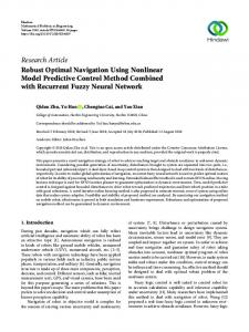
where u1 (k), u2 (k), y(k) and e(k) are the inputs, the output and the model error respectively. The model error is assumed to be bounded such |e(k)| ≤ 4.51 and the input signals are uniformly distributed sequences. In this simulation we approximate this model by the GOBF model where the truncating order and the optimal poles are: Nopt = 4; ξopt = (0.7450 0 0.3547 − 0.7047). The process output and the GOBF model output are illustrated in figure 1. 25

Process output GOBF model output

20

10

0

−10

−20 0

100

200

300

Figure 1: Process output and GOBF model output The center and uncertainty intervals (UI) of the ellipsoid are given in table 1. The tuning parameters used in this simulation are: h2 = 8, hu = 2, λ1 = 1 and λ2 = 1. Table 1: Ellipsoid Performances Ellipsoidal center -0.6326 -0.9135 -0.2266 Uncertainty intervals 0.3797 0.9320 0.7085

-0.1260 1.9076

To validate the control method we plot in figure 2 the GOBF model output and the reference signal. The control signals and the control increment signals are illustrated in figure 3 and 4 successively. The picks of the control signals as well as the control increment signals are due to the changed reference signal from -40 to +40 at the iterations 100 and 200. Therefore, we notice the rapid convergence of the model output to the reference signal. This is predictable since we optimize a tracking criterion. Other simulation examples with different GOBF models and reference signals have been studied and yielded the same results.

362


50 40

GOBF model output Reference signal

0

−40 −50 0

100

200

300

Figure 2: Reference signal and GOBF model output 40

10 Control signal u1

Control signal u2

30 5 20

10

0

0 −5

−10

−20 −10 −30

−40 0

100

200

300

−15 0

100

200

300

Figure 3: Control signals 25

25 Control increment signal 2

Control increment signal 1 20

20

15

15

10

10

5 5 0 0 −5 −5 −10 −10

−15

−15 −20 0

−20

100

200

300

−25 0

100

Figure 4: Control increment signals

200

300


363

On the other hand, the influence of the error bounds on the GOBF model output in the case of an ellipsoid domain is studied by considering 3 different SNR (signal to noise ratio). The table 2 gives the centers and the uncertainly intervals where the figure 5 illustrates the model outputs and the reference signal fixed arbitrary. This figure shows the similar convergence of the model outputs to the reference signal. Thus, we conclude that for different error bounds, we obtain the same GOBF model output. The control method has been tested with different reference signals and error bounds that yielded the same results. Finally we study the influence of different uncertainty domains such an ellipsoid, an orthotope and a polytope. The table 3 regroups the centers and the uncertainty intervals of these domains. The model outputs correspondent are shown in figure 6. By examining this figure we notice that the model outputs converge simultaneously to the reference signal. So, we conclude that the type of the parameter domain has no influence on this control method. Other experiences with different reference signals and domain parameter have been realized and yielded the same results. Table 2: Ellipsoid performances for different error bounds SNR=5 Center -0.5698 -1.0975 -0.2557 -0.0844 UI 0.7915 1.9507 1.4634 3.9237 SNR=10 Center -0.6071 -0.9886 -0.2377 -0.1086 UI 0.5517 1.3550 1.0246 2.7549 SNR=20 Center -0.6326 -0.9135 -0.2266 -0.1260 UI 0.3797 0.9320 0.7085 1.9076

Table 3: Domain performances (SNR=20) Center -0.6326 -0.9135 -0.2266 UI 0.3797 0.9320 0.7085 Orthotope Center -0.6950 -0.7551 0.1082 UI 0.6403 1.6896 1.7069 Polytope Center -0.6924 -0.7556 -0.1968 UI 0.0236 0.0307 0.0472 Ellipsoid

-0.1260 1.9076 -0.1356 4.2133 -0.1754 0.1095

60 50

0

GOBF model output (SNR=20) GOBF model output (SNR=10) GOBF model output (SNR=5) Reference signal −50 −60

0

100

200

300

Figure 5: Model outputs for 3 different SNR of an ellipsoid domain

364


40 GOBF model output (Ellipsoid) GOBF model output (Orthotope) GOBF model output (Polytope) Reference signal

30

0

−30

−40

0

150

300

Figure 6: Model outputs for different uncertainty domains

6

Conclusion

This paper has presented a new robust predictive control method based on the GOBF model for a MISO system. A min-max problem is solved taking into account the uncertainties on the model coefficients and the constraints on the control signals. The uncertainty parameter domain can be an ellipsoid, an orthotope or a polytope and the performance criterion is optimized with respect to constraints relative to parameter uncertainties and measurement constraints. The implication of these results in the context of system controls is that the GOBF can be used to deliver state space models suitable to synthesize a robust predictive control without affecting the computational complexity and the performance of the method. Finally, it should also be noted that this control method provides best results and may be synthesized for a MIMO system represented on the GOBF.

Bibliography [1] G. Oliveira, G. Favier, G. Dumont, and W. Amara, Predictive Controller Based on Laguerre Filters Modeling, In Proc. 13th IFAC World Congress, San Francisco, USA, vol. G, pp. 375-380, 1996. [2] A. Mbarek, H. Messaoud and G. Favier, Robust predictive control using Kautz model, In Proc. 10th IEEE International Conf. Electronics, Circuits and Systems, pp. 184-187, December 2003. [3] L.P. Wang, Discrete time model predictive control design using Laguerre functions, Journal of Process Control, 14:131-142, 2004. [4] E.M. El Adel, M. Ouladsine, and L. Radouane, Predictive steering control using Laguerre series representation, In Proc. 2003 American Control Conf., vol.1, pp. 439-445, June 2003. [5] B. Wahlberg, System identification using Laguerre models, IEEE Trans. on Automatic Control, 36(5): 551-562, 1991. [6] B. Wahlberg, System identification using Kautz models, IEEE Trans. on Automatic Control, 39(6):1276-1282, 1994. [7] A. Gutierrez and E. Camacho, Robust Adaptive Control for Processes with Bounded Uncertainties, In Proc. 3rd ECC, Roma, vol.2, pp. 1295-1300, 1995.


365

[8] J. Ghabi, A. Douik and H. Messaoud, A New Modelling Approach of MIMO linear Systems using the generalized Orthonormal basis functions, In Proc. of the 6th ISPRA’07, Greece, pp. 192-196, February 2007. [9] J. Ghabi, A. Douik and H. Messaoud, New Methods of Modelling and Parameter Estimation for MIMO linear Systems using Generalized Orthonormal Basis Functions, Journal on Systems and Control, vol. 2, pp. 133-140, 2007. [10] B. Ninness and F. Gustafsson, A unifying construction of orthonormal bases for system identification, IEEE Trans. on Automatic Control, 42 (4): 515-521, 1997. [11] P. S. C. Heuberger, P. M. J. Van den Hof, and O. H. Bosgra, A generalized orthonormal basis for linear dynamical systems, IEEE Trans. on Automatic Control, 40(3):451-465, 1995. [12] Paul Van den Hof, Brett Ninness, System Identification with Generalized Orthonormal Basis Functions, In Modelling and Identification with Rational Orthogonal Basis Functions, Springer Verlag, chap.4, pp. 61-102, 2005. [13] G. Favier and L. Arruda, Review and Comparison of Ellipsoidal Bounding Algorithms, In M. et al., editor, Bounding Approaches to system identification, Plenum Press, New York, chap.4, pp. 43-68, 1996. [14] H. Messaoud and G. Favier, Recursive determination of parameter uncertainty intervals for linear models with unknown but bounded errors, In Proc. 10th IFAC Symposium on System Identification, Copenhagen, Denmark, pp. 365-370, 1994. [15] S. Maraoui and H. Messaoud, Design and comparative study of limited complexity bounding error identification algorithms, IFAC, Symposium on System Structure and Control, Prague, Cheque Republique, pp. 29-31, 2001. [16] J. Ghabi, A. Douik and H. Messaoud, A New Estimation Method of the Poles for the generalized Orthonormal bases filters, In Proc. of the 6th ISPRA’07, Greece, pp. 197-202, February 2007. [17] J. Ghabi, A. Douik and H. Messaoud, A New Technique of Poles Estimation for Generalized Orthonormal Basis Functions, Journal on Systems and Control, vol.2, pp. 125-132, 2007. Ali Douik, Jalel Ghabi and Hassani Messaoud Ecole Nationale d’Ingénieurs de Monastir (ENIM) Département de Génie Electrique Laboratoire ATSI Rue Ibn El Jazzar, 5019 Monastir Tunisie E-mail: [email protected], [email protected], [email protected] Received: June 30, 2007

366


Ali Douik was born in Tunis, Tunisia. He received the Master degree in 1990 and the Ph.D. degree in 1996 of science Electrical Genius from the “Ecole Normale Supérieur de l’Enseignement Technique de Tunis”. He is currently “Maitre assistant”in the “Ecole Nationale d’Ingénieurs de Monastir”and Director of the “Département de Génie Electrique”. His research is related to Signal Processing and Automatic Control.

Jalel Ghabi was born in Kairouan, Tunisia. He received the diploma of Graduate Engineer in Electrical Genius from the “Ecole Nationale d’Ingénieurs de Monastir”, in 1997. He obtained her Master of Automatic and Industrial Data Processing from “Ecole Nationale d’Ingénieurs de Sfax”, in 2003. He is currently preparing the PhD. Degree in Control Automatic in the laboratory ATSI “Automatique, Traitement de Signal et Imagerie”. His research is related to the Robust Predictive Control of MIMO systems using Generalized Orthonormal Basis Functions. Hassani Messaoud was born in Mahdia, Tunisia. He received the Master degree from the “Ecole Normale Supérieur de l’Enseignement Technique de Tunis”, in 1985 and the Ph.D. degree in Automatic Control from the “Ecole Centrale de Lille, France”, in 1993. In 2001, he received the ability degree from the “Ecole Nationale d’Ingénieurs de Tunis”. He is presently Professor in the “Ecole Nationale d’Ingénieurs de Monastir”and Director of the laboratory ATSI. He has been the supervisor of several PhD thesis and is author or co-author of several Journal articles. His research is related to Automatic Control and Signal Processing.