Linear programming-based robust model predictive control for positive

IET Control Theory & Applications Research Article

Linear programming-based robust model predictive control for positive systems

ISSN 1751-8644 Received on 14th February 2016 Revised 7th April 2016 Accepted on 3rd May 2016 E-First on 2nd August 2016 doi: 10.1049/iet-cta.2016.0149 www.ietdl.org

Junfeng Zhang1 , Xudong Zhao2, Yan Zuo3, Ridong Zhang3 1Institute

of Information and Control, Automation, Hangzhou Dianzi University, Hangzhou 310018, People's Republic of China of Electronic Information and Electrical Engineering, Dalian University of Technology, Dalian 116024, People's Republic of China 3Key Lab for IOT and Information Fusion Technology of Zhejiang, Hangzhou Dianzi University, Hangzhou 310018, People's Republic of China E-mail: [email protected]

2Faculty

Abstract: This study investigates the problem of robust model predictive control for positive systems under a new model predictive control framework. A robust model predictive control method is presented in this study for uncertain positive systems. A state-feedback control law that robustly stabilises the underlying system is designed by using linear programming. Different from the traditional model predictive control technique, the authors' proposed model predictive control framework employs a linear infinite horizon objective function and a linear Lyapunov function rather than quadratic performance indices and quadratic Lyapunov functions commonly used in the literature. Compared with existing design techniques for positive systems, the present approach owns the following advantages: (i) it gives a locally optimal control strategy which approaches to actual operation conditions and the control law is designed by solving a locally optimal control problem at each time step, (ii) it can explicitly deal with constraints of the systems, and (iii) the controller can be easily designed via linear programming without any additional constraints. An practical example is provided to verify the validity of the theoretical findings.

1 Introduction Over the past two decades, positive systems have drawn much attention [1–7] due to their theoretical significance and extensive applications in engineering. Positive systems possess many special, but nice features, for instance, positive systems hold the signpreserving property, that is, the states always stay in the positive or negative orthants whenever the initial conditions take non-negative or non-positive values, respectively; the stability of a positive timedelay system is not effected by the time-delay if the time-delay is bounded and so on. Due to the special features of positive systems, many traditional approaches cannot be applied to positive systems [1, 2]. In the early time of this century, the works [1, 2] described the fundamental properties of positive systems and presented some constructive criteria on controllability, reachability, observability and so on. The authors in [8] constructed a linear copositive Lyapunov function for positive systems, which was used to discuss the stability of positive systems [9–12]. Ait Rami et al. for the first time, addressed a linear programming technique to the stabilisation of positive systems [13, 14], which was further used to investigate the output-feedback control [15], ℓ1-induced control [16], robust stabilisation [17] and so on [18–21]. At present, the linear copositive Lyapunov function associated with the linear programming technique is often applied to positive systems though there are some other techniques [22, 23]. As we all know, an optimal or suboptimal control design of a system is always a hot topic. There have been many results on optimal or suboptimal control design approaches for various control systems [24–27]. Regrettably, the optimal and suboptimal control designs of positive systems have rarely been studied in the literature [28, 29]. It is necessary to state two points. First, the work [29] mainly discussed the open-loop optimal stability of positive systems since the control vector was imposed on the system matrix. Second, there exist some limitations in [28] to guarantee the positivity of the closed-loop systems when linear matrix inequality was employed. These observations imply that the optimal and suboptimal control designs of positive systems still keep open.

IET Control Theory Appl., 2016, Vol. 10 Iss. 15, pp. 1789-1797 © The Institution of Engineering and Technology 2016

This paper tries to address a robust model predictive control (RMPC) approach to constrained positive systems. The motivations of this paper are inspired by the two aspects. From the theoretical viewpoint, it has been verified that RMPC is powerful for dealing explicitly with the constraint problems of a control system [30–33]. RMPC employs a prediction model of a plant to optimise the future plant behaviour, and the optimisation procedure is performed at each time step. This property of RMPC ensures that the designed state behaviour satisfies the desired requirements. Therefore, RMPC is often chosen to solve the constraint problems of some systems. However, up to now, there has been few efforts devoted to RMPC for positive systems. As the first attempt, we address RMPC for positive systems in [34]. The results in [34] also reveal that RMPC is effective for positive systems as it is for nonpositive systems. This paper is a continuation of [34]. From the viewpoint of practical applications, it is important to investigate the RMPC for positive systems. Positive systems can be used to describe the TCP-like congestion control [4]. Assume that a control vector is added to the TCP-like congestion control model. How to predict the future congestion status by the present network status? How to design a control strategy to reduce congestion and guarantee the normal operation of the networks? These aspects are important and useful for reducing network congestion. The readers can refer to [1, 2, 35, 36] for more examples. By observing the properties of RMPC, it has potential applications in positive systems. This paper addresses an RMPC for constrained positive systems. First, a linear copositive Lyapunov function is constructed. By using the linear Lyapunov function, a statefeedback controller is designed via linear programming, under which the computation burden (online and offline) is low. Here, it is necessary to point out that linear programming is more effective than linear matrix inequality when dealing with large-scale computation. This makes linear programming hold powerful capability to solve the computation of RMPC for positive systems. Compared with existing RMPC, the difficulties of the design in this paper lie in: (i) how to address a proper performance index function according to a linear copositive Lyapunov function, (ii) how to design an invariant set, and (iii) how to transform the control design conditions into linear programming. The remaining 1789

of this paper is organised as follows: the problem statement is formulated in Section 2. Section 3 addresses the design process of RMPC. An illustrative example is provided in Section 4. Section 5 concludes the paper. Notations: Denote by ℜ, ℜ�, ℜ� × � the set of real numbers, the set of �-dimensional vectors, and the space of � × � matrices, respectively. The symbols ℕ and ℕ+ represent the non-negative and positive integers, respectively. �� denotes to the convex hull. For � ∈ ℕ+, denote by � := {1, 2, …, �}. Denote by ��( ⋅ ) the vector operation, which consists of the columns of a matrix taken from left to right and stacked one above the other. Let ⨂ be the Kronecker product. A matrix � represents the identical matrix with proper dimension. For a vector �, � ⪰ 0 (� ≻ 0) means that all its components �� ≥ 0 (�� > 0). For a matrix �, � ⪰ 0 (� ≻ 0) means that all its �th row �th column components �� ≥ 0 (�� > 0). Furthermore, � ⪰ � (� ≻ �) means that �� ≥ �� (�� > ��), where �� and �� are the �th row �th column components of matrices � and �, respectively. Define �� = (1, …, 1)T and �

��(�) = (0, …, 0, 1, 0, …, 0)T. The Euclidean norm and 1-norm of a

vector

�−1

� ∈ ℜ�

�−�

are

defined

by

Σ��= 1 | ��|.

| | � | |2 = 2 Σ��= 1��2

and

| | � | |1 = Throughout this paper, the dimensions of matrices and vectors are assumed to be compatible if they are not stated.

2 Problem statement Consider the following linear time-varying system: �(� + 1) = �(�)�(�) + �(�)�(�),

(1)

where �(�) ∈ ℜ� is system state and �(�) ∈ ℜ� is control input. The system matrix [�(�) �(�)] is assumed to be located in a prescribed uncertain set. In this paper, two types of uncertain sets Ω are considered. The first uncertain set is interval uncertainty satisfying Ω1 := {[�(�) �(�)]: � ⪯ �(�) ⪯ �, � ⪯ �(�) ⪯ �, ∀� ∈ ℕ}

(2)

Ω2 := co{[�1 �1], [�2 �2], …, [�� ]},

(3)

and the second one is polytope uncertainty satisfying

which means that there exist � non-negative real numbers ��, � ∈ � such that [�(�) �(�)] =

�

∑ ��[�� ],

�=1

∀� ∈ ℕ

where ∑�� = 1 �� = 1, �� ≥ 0 and �� ∈ ℜ� × �, �� ∈ ℜ� × � . constraint on the gain matrix of the controller is given as | | �T�� | |1 ≤ �,

(4) The

(5)

where � is the gain matrix of the controller to be designed and � ≥ 0. The models (1) with (2) and (1) with (3) are called interval systems and polytopic systems, respectively. Polytopic systems employ the different operation model at different times or different status as their vertices. Therefore, this class of systems is suitable for describing time-varying systems and non-linear systems and has been extensively considered in the RMPC problems [30–34]. Interval systems are much easier to describe an uncertain control system than polytopic systems because interval systems only need to give an interval rather than an explicit description of systems. For general systems (non-positive), the control design of interval systems is much harder than the one of polytopic systems. For positive systems, interval uncertain systems possess nice 1790

properties, for instance, the positivity and stability of the two endpoints can guarantee the positivity and stability of interval systems. These properties are helpful for reducing the difficulties of the control design. So, we address the model (1) with (2). Being different from the conditions in the RMPC literature, we utilise 1-norm in (5) to describe the constraint conditions. Positive systems often characterise the number of population, the amount of the materials and so on. Therefore, the 1-norm is suitable for describing these quantities. Especially, the condition (5) only imposes the constraint on the gain matrix and there is not any constraint on the states and output. We will explain the reason later (see Remark 6). In order to satisfy the positivity requirement of positive systems, we introduce two additional assumptions to the system matrices as follows: Assumption 1: � ⪰ 0 and � ⪰ 0. Assumption 2: �� ⪰ 0 and �� ⪰ 0 ∀� ∈ �. Next, we provide some preliminaries about positive systems for later developments. Definition 1 (1,2): A system is positive if its states and outputs are non-negative (i.e. �(�) ⪰ 0 and �(�) ⪰ 0) for any nonnegative initial conditions (i.e. �(�0) ⪰ 0) and any non-negative control input (i.e. �(�) ⪰ 0). Lemma 1 (1,2): A system �(� + 1) = ��(�) + ��(�)

(6)

is positive if and only if � ⪰ 0 and � ⪰ 0. Lemma 2 ([1,2]): Given a matrix � ⪰ 0 with � ∈ ℜ� × �, then the following statements are equivalent: i. The matrix � is a Schur matrix. ii. There is a vector � ≻ 0 in ℜ� such that (� − �)� ≺ 0.

Definition 2: A function �(�) = �(�)T� is called as a linear copositive Lyapunov function of the system (6) with �(�) = 0 if there exists a vector � ∈ ℜ� with � ≻ 0 such that (� − �)T� ≺ 0. Remark 1: For a positive system (6), assume � is not a Schur matrix, i.e. the open-loop system is unstable by Lemma 2. Then, we have the fact: there does not exist a controller gain matrix � ⪰ 0 such that the control law �(�) = ��(�) stabilises the system. We confirm the fact via a simple deduction. Suppose that there exists a gain matrix � ⪰ 0 such that the closed-loop system is stable, then there exists a vector � ≻ 0 such that (� + �� − �)� ≺ 0 by Lemma 2. This together with � ⪰ 0 and � ⪰ 0 gives (� − �)� ≺ 0, which implies that � is a Shur matrix. This contradicts with the prerequisite. So, the stabilisation for a positive system can be interpreted as designing a non-positive control law such that the resulting closed-loop system is positive and stable. This point has also been stated in [14, 15]. In this paper, we have the following statement: Statement 1: State-feedback control laws to be designed are required to be negative. Remark 2: Aiming to the introduction of a new RMPC cost function in Section 3, Statement 1 is addressed. In addition, the fact in Remark 1 also implies that Statement 1 is necessary. It should be pointed out that there may exist a state-feedback control law with non-positive and non-negative components such that the system is stable. Lemma 3 (14): Given a positive system �(� + 1) = ��(�), then 0 ⪯ �(�) ⪯ � for any initial condition satisfying 0 ⪯ �(�0) ⪯ � if and only if (� − �)� ≺ 0. IET Control Theory Appl., 2016, Vol. 10 Iss. 15, pp. 1789-1797 © The Institution of Engineering and Technology 2016

3 Main results This section is divided into two subsections. The first subsection is devoted to addressing a new linear cost function and the second subsection present the RMPC controller design.

In this subsection, we will present a new linear cost function for the RMPC of positive systems by following the classic RMPC approach. RMPC is a step-by-step optimisation technique. At each sampling time, a state-feedback controller is designed to minimise the cost function depending the future states. In this paper, we aim to achieve the following performance index: min

�(� + � | �), � ∈ ℕ

�∞(�) :=

max

[�(� + �) �(� + �)] ∈ Ω, � ∈ ℕ

3.1 Cost function

with

As those cost functions commonly used in the literature, it is assumed that (8) is well-defined. This implies that �∞(�) is bounded. Thus, �(�) → 0 as � → ∞. Therefore, we have

max

[�(� + �) �(� + �)] ∈ Ω, � ∈ ℕ

�∞(�)

∞

∑ (�(� + � | �)T� + �(� + � | �)T�)

(7)

(8)

�=0

where �(� + � | �) and �(� + � | �) are the future state and control law predicted at time �, � ≻ 0 with � ∈ ℜ�, and � ≺ 0 with � ∈ ℜ�. Note from (8) that the cost function used for the considered systems is linear whereas the one for general systems is always chosen as a quadratic form: (see (9)) where � and � are positive definite matrices. The choice of linear cost function (8) comes from two reasons. First, it is based on the essential properties of positive systems. For positive systems, it is always required that �(�) ⪰ 0. In addition, �(�) ⪯ 0 by Statement 1. Thus, the cost function (8) is more suitable to describe the performance index than (9). Furthermore, the state of positive systems often represents the number of population or insect population, the total amount of material and so on. It is better to describe these quantities via the linear form (8) than the quadratic form (9). This paper will consider RMPC of positive systems by employing a linear copositive Lyapunov function associated with linear programming technique. Accordingly, a linear cost function is more proper than a quadratic form. Second, the cost function (8) is a natural development of (9). Positive systems possess many special features, which require the introduction of new approaches. For instance, a linear copositive Lyapunov function is constructed for positive systems, linear programming technique is used, the classic �2-gain performance is extended to �1-gain performance of positive systems [16, 17] and so on. Similarly, a linear cost function (8) is introduced for RMPC of positive systems. The objective of the paper is to design a linear programming based state-feedback control law �(� + � | �) = ��(� + � | �), � = 0, 1, …, �, minimising the cost function (8), where � is the predicted steps. For the objective, a linear copositive Lyapunov function is constructed as follows: �(�, �) = �(� + � | �)T�,

(10)

where � ≻ 0 with � ∈ ℜ� . At each sampling time, an additional condition is imposed on the Lyapunov function in the following form: (see (11)) Summing both sides of (11) from 0 to ∞ gives max

[�(� + �) �(� + �)] ∈ Ω, � ∈ ℕ

�∞(�) ≤ �(0, �) − �(∞, �) .

�∞(�) :=

(12)

�∞(�) ≤ �(0, �) .

(13)

Noting the performance index (7) and the condition (13), the objective of (7) can be gotten by resorting to the condition �(0, �) = �(� | �)T� ≤ �

(14)

with (11), where � ≥ 0 is a variable to be minimised. Remark 3: By Statement 1, �(�) ⪯ 0. This together with � ≺ 0 in (8) gives �∞(�) ≥ 0. Thus, (13) and (14) are valid. If �∞(�) < 0, then (13) is meaningless. This will lead to that an optimisation problem to � in the later section is not valid. In addition, assume �(� + � | �)T� < 0, then it may deduce that �(� + � | �)T� + �(� + � | �)T� < 0. So, �(� + 1, �) > �(�, �). This will destroy the stability of the system. These are why we address Statement 1 and choose the cost function (8). 3.2 RMPC design In this subsection, we will propose the RMPC design for system (1) with (2) and system (1) with (3), respectively. Then, a cone invariant set is introduced for RMPC. We first give Lemma 4 to solve the controller design for system (1) without constraints. Lemma 4 ((control law)): Consider system (1) with (2) and system (1) with (3) without constraints. Let �(� | �) be the measured state �(�). a.

For system (1) with (2) under Assumption 1, there exist vectors � ≻ 0 with � ∈ ℜ�, �(�) ∈ ℜ�, � ≺ 0 with � ∈ ℜ�, � ≻ 0 with � ∈ ℜ� and a constant � > 0 such that �T� + � − � + � ≺ 0,

��T� � + �

and

�

∑ �� ⪰ 0,

(15a)

( ) ( )

(15b)

�T� + � ⪰ �,

(15c)

�=1

�(�) ≺ �,

(15d)

�(� | �)T� ≤ �,

(16)

�T� + � − � + � ≺ 0,

(17a)

hold ∀� ∈ �, or there exist vectors � ≻ 0 with � ∈ ℜ�, �(�) ≻ 0 with �(�) ∈ ℜ�, � ∈ ℜ�, � ≺ 0 with � ∈ ℜ� and a constants � > 0 such that ��T� � + �

( ) ( )

(17b)

�T� + � ⪰ �,

(17c)

�=1

∞

∑ (�(� + � | �)T��(� + � | �) + �(� + � | �)T��(� + � | �))

�

∑ �� ⪯ 0,

(9)

�=0

�(� + 1, �) − �(�, �) ≤ − [�(� + � | �)T� + �(� + � | �)T�], ∀[�(� + �) �(� + �)] ∈ Ω .


(11) 1791

�T� + � ⪯ 0,

(17d)

�(�) ≺ �,

a.

(17e)

From � ≻ 0 and (15b), we can get

and (16) hold ∀� ∈ �, then under the state-feedback control law �(� + � | �)

b.

= ��(� + � | �) =

Σ�� = 1�(��)�(�)� �T� �

�(� + � | �)

�+�

(18)

+ � − � + � ≺ 0,

� ��T� � + � �

�

∑ �� ⪰ 0,

�=1

( ) ( )

�T� � + � ⪰ �,

(20a)

� ��T� � + � �

∑ �� ⪯ 0,

(20b)

+ � ⪯ 0,

(20d)

�=1

( ) ( )

�T� � + � ⪰ �,

�T� �

�(�) ≺ �,

(20c)

(20e)

and (16) hold ∀(�, �) ∈ � × �, then under the state-feedback control law �(� + � | �)

= ��(� + � | �) =

Σ�� = 1�(��)�(�)� �T� �

�(� + � | �)

Proof: We give the proofs of (15), (16), (18) and (19), (16), (21). The proofs of (17), (16), (18) and (20), (16), (21) can be gotten by a similar method and are omitted.

(23)

� + �� ⪰ � + �� ⪰ 0.

(24)

(25)

It follows from (15c) and � ≻ 0 that �T� + � ≻ 0, which together with (15d) gives (see (26) and (27)) By (15c), we can obtain that �T� (�T� + �) ⪰ �T� � . Thus, �T(�T� + �) ⪯ �. By (15a), we have (see (27)) By Assumption 1 and � ≺ 0, we get 0 ≻ �T� + �T�T� + �T� − � + �

≻ �T� + �T�T� + �T� − � + �,

b.

(28)

which implies that (25) holds. This means that the condition (11) is valid. In addition, the condition (14) can be guarantee by using (16). The proof is provided via a three-step process. In the first step, we prove that system (1) is positive under the statefeedback control law (21). Consider each vertex system of system (1) �(� + 1) = � ��(�) + � ��(�),

� ∈ �.

(29)

Then, under the state-feedback control law (21), the resulting closed-loop system is �(� + 1) = (� � + � ��)�(�)

(21)

system (1) with (3) is positive and the conditions (11) and (14) are satisfied.

� + �� ⪰ 0.

�T� + �T�T� − � + � + �T� ≺ 0.

and (16) hold ∀(�, �) ∈ � × �, or there exist vectors � ≻ 0 with � ∈ ℜ�, �(�) ≻ 0 with �(�) ∈ ℜ�, � ∈ ℜ�, � ≺ 0 with � ∈ ℜ� and a constant � > 0 such that �

(22)

Choose a linear copositive Lyapunov function as (10). Owing to �(�) ⪰ 0 ∀� ∈ ℕ, the condition (11) holds if

(19c)

�T� � + � − � + � ≺ 0,

⪰ 0.

By Lemma 1, the resulting closed-loop system (1) with the control law (18) is positive, i.e. �(�) ⪰ 0 ∀� ∈ ℕ.

(19b)

(19d)

�T� �

Since � ≻ 0, � ≺ 0, and (15d), then � ≺ 0. Thus, Statement 1 is satisfied. With the condition (2) and Assumption 1 in mind, we have

(19a)

�(�) ≺ �,

Σ�� = 1��(�)�

From (18) and (22), we have

system (1) with (2) is positive and the conditions (11) and (14) are satisfied. For system (1) with (3) under Assumption 2, there exist vectors � ≻ 0 with � ∈ ℜ�, �(�) ∈ ℜ�, � ≺ 0 with � ∈ ℜ�, � ≻ 0 with � ∈ ℜ� and a constant � > 0 such that �T� �

The proof is give via a two-step strategy. In the first step, we prove that the resulting closed-loop is positive. In the second step, we prove that the conditions (11) and (14) are satisfied.

= �� + ��

Using � ≻ 0 and (19b) gives

�� + ��

Σ�� (�)� �T� �

Σ�� (�)� �T� �

�(�), � ∈ � .

⪰ 0,

(30)

(31)

which means that the resulting closed-loop system (29) for each � ∈ � is positive by Lemma 1. Thus, the closed-loop

�T(�T� + �) =

1792

∑�� = 1 �(�)��(�)�(�T� + �)

∑�� = 1 ��(��)�(�T� + �)

(26)

0 ≻ �T� + � − � + � ⪰ �T� + �T(�T� + �) − � + � = �T� + �T�T� + �T� − � + �,

(27)

�T� �

=

��T� (�T� + �)

.

�T� �

⪯

�T� �


system (1) under the control law (21) is positive, i.e. �(�) ⪰ 0 ∀� ∈ ℕ.

In the second step, we prove that for system (29), the conditions (11) and (14) are satisfied under (19), (16), and (21). Choose a linear copositive Lyapunov function �(�, �) as (10). The condition (11) holds if �(� + � | �)T

�T� � + �T�T� � − � + � + �T� < 0.

By �(� + � | �) ⪰ 0, the condition (32) is equivalent to �T� � + �T�T� � − � + � + �T� ≺ 0.

(32)

(33)

By � ≺ 0 and (19d), we have �(�) ≺ 0. This together with � ≻ 0 gives � ≺ 0, which implies that Statement 1 is satisfied. Furthermore, we have (see (34)) Using (19c) gives ��(�T� � + �) ⪰ �T� � . Thus, �T�T� � + �T� ≺ �. Noting (19a), we get 0 ≻ �T� � + � − � + �

≻ �T� � + �T�T� � − � + � + �T�

(35)

which verifies (33). In addition, the condition (16) can guarantee the validity of (14). □ Finally, we prove that for system (1), the conditions (11) and (14) are also satisfied under the conditions (19), (16), and (21). First, the condition (14) can be directly obtained by (16). By (4), we have [�(� + �) �(� + �)] = Σ�� = 1� �(� + �)[� � � �]. Multiplying both sides of (19) by � �(� + �) and then summing them from � = 1 to � yields �(� + �)T� + � − � + � ≺ 0, �(� + �)�T� � + �(� + �) T

�(� + �) � + � ⪰ �,

�

∑ �� ⪰ 0,

�=1

( ) ( )

∑�� = 1 �(�)��(�)�(�T� � + �) �T� �


a.

For system (1) with (2), suppose that (15) [or (17)] holds. If the condition

(36)

Using the same proof as that in the second step, it is easy to get that the conditions (11) and (14) are also satisfied for system (1). Remark 4: In Lemma 4, a single-step control strategy is employed to solve the RMPC design of uncertain positive systems by following the approach in [30]. As we all know, the single-step control approach exists conservativeness. For non-positive systems, some improved RMPC approaches such as the parameterdependent Lyapunov functions approach [32, 33] and the multiplestep control approach [34] have been addressed. These improved approaches are more efficient than the single-step control approach. A natural idea is: whether these improved approaches can be extended to the RMPC of positive systems. The answer may be positive. However, we failed to complete the extension. In our opinion, the difficulty mainly lies in how to guarantee the convexity of the present conditions. How to present more efficient RMPC approaches for positive systems is an interesting topic in future work. Remark 5: Lemma 4 proposes the model predictive control laws for positive systems. From the proof of Lemma 4, we can get that the proposed design is also suitable for non-positive systems, i.e. Assumptions 1 and 2 are removed. That is to say, for a system, if there exists a non-negative state-feedback control law such that the

�T(�T� � + �) =

resulting closed-loop system is positive and stable, then Lemma 4 is available. It is worthy noting that not all systems satisfy the aforementioned condition. Meanwhile, what class of systems admits the positivity of their closed-loop systems under a nonnegative state-feedback control law is still an open problem. The following algorithm can be used to get an optimal value of �: Algorithm 1 min�, �, � � is subject to (15) or (17) and (16) [or, (19) or (20) and (16)]. We are in a position to introduce an invariant set for RMPC of positive systems in Lemma 5, which will also be required to prove the stability of the system. Lemma 5 ((invariant set)): Suppose (15) or (17) [or, (19) or (20)] holds for system (1) with (2) (or, (1) with (3)) with the control law (18) [or, (21)]. Then, �(� | �)T� ≤ � implies max[�(� + �) �(� + �)] ∈ Ω, � ∈ ℕ �(� + � | �)T� ≤ �, � ∈ ℕ+. Proof: From the proof of Lemma 4, we know that the condition (11) holds, i.e, �(� + 1, �) − �(�, �) ≤ 0. Then, �(� + � + 1 | �)T� ≤ �(� + � | �)T� ≤ �. This means that if �(� | �)T� ≤ �, then �(� + 1 | �)T� ≤ �. By induction, + T �(� + � | �) � ≤ � ∀� ∈ ℕ . □ If Lemma 5 holds, then the set ℑ = {� | �T� ≤ �} is called a cone invariant set for RMPC of positive systems. In the literature, an ellipsoid is often chosen as the invariant set for RMPC of general systems. In this paper, the linear copositive Lyapunov function associated with linear programming technique is employed. Accordingly, a cone is introduced to describe the invariant set of RMPC. In order to handle the system constraint, we present Lemma 6 to incorporate the condition (5) into linear programming. Lemma 6 ((constraint)): Consider system (1) with (2) and system (1) with (3) under the constraint condition (5).

⪯

��T� � + �T�

b.

�

∑ ��

�=1

( )

≥ 0 (�� ≤ 0)

(37)

≥ 0 (�� ≤ 0)

(38)

holds, then under the control law (18) the constraint condition (5) is satisfied. For system (1) with (3), suppose that (19) [or (20)] holds. If the condition ��T� � + �T�

�

∑ ��

�=1

( )

holds ∀� ∈ �, then under the control law (21) the constraint (5) is satisfied.

Proof: a.

By (15c), it follows that: �+

�T�Σ�� = 1�(�) T �� (�T� � + �)

≥ 0.

Using the fact �T� ��(�) = 1 and � ≺ 0, we have (see (39)) This implies that the constraint condition (5) is satisfied for system (1) with (2) when (15) holds.

∑�� = 1 ��(��)�(�T� � + �) �T� �

=

��(�T� � + �) �T� �

.

(34) 1793

Take (17) into account. By (17c) and (17d), we have �+

b.

�T�Σ�� = 1�(�)

�T� (�T� � + �)

≥ 0.

Similar to the proof of (39), we can get that the constraint condition (5) is satisfied for system (1) with (2) when (17) holds. The proof can be provided by using a similar method to that in (a) and is omitted. □

Remark 6: In the traditional RMPC design, the constraint conditions are usually imposed on the state �(�), the output �(�), and the control law �(�). The condition (5) only imposes the constraint on the gain matrix of the control law. In the following, we discuss this point in detail. Since � ≺ 0 and � ≺ 0, �T� ≻ 0. Noting (28), (33), and � ≻ 0, we get that there exists a vector � ≻ 0 such that (� + �� − �)T� ≺ 0. Given a matrix � ⪰ 0, it is true that if there exists a vector � ≻ 0 such that (� − �)� ≺ 0, then there must exist a vector �′ ≻ 0 such that (� − �)T�′ ≺ 0 vice versa. Combining this fact with Lemma 3, we have that for a positive system �(� + 1) = ��(�), if there exists a vector � ≻ 0 such that (� − �)T� ≺ 0, then 0 ⪯ �(�) ⪯ � ∀� ∈ ℕ holds for any initial conditions satisfying 0 ⪯ �(�0) ⪯ �. Consider system (1) with (2) and system (1) with (3). The states satisfy 0 ⪯ �(�) ⪯ � ∀� ∈ ℕ with any initial conditions satisfying 0 ⪯ �(�0) ⪯ � owing to (� + �� − �)T� ≺ 0. Arbitrarily given an initial condition �(�0), there must exist a constant ℏ > 0 such that 0 ⪯ �(�0) ⪯ ℏ�. Therefore, we can deduce that the states of system (1) with (2) and system (1) with (3) satisfy 0 ⪯ �(�) ⪯ ℏ� ∀� ∈ ℕ for any initial condition satisfying 0 ⪯ �(�0) ⪯ ℏ�, where ℏ > 0. Based on the discussions above, we get that the bound of the state �(�) depends on the bound of the initial condition �(�0). In general, the initial condition is known. Thus, the output also depends on the initial condition �(�0) when the weight matrix of the output is known. These points mentioned above are why the constraint condition (5) is used in this paper. Theorem 1: Let �(�) = �(� | �) be the measurable state of system (1) at sampling time �. a.

b.

Consider systems (1) and (2) under Assumption 1. Under the control law (18), the upper bound �(�, �) of the robust performance objective function is minimised and the constraint (5) is satisfied. The state-feedback gain matrix can be obtained by solving the following optimisation problem: min � subject to (15) or (17), (16), and (37). �, �, �

Consider system (1) with (3) under Assumption 2. Under the control law (21), the upper bound �(�, �) of the robust performance objective function is minimised and the constraint (5) is satisfied. The state-feedback gain matrix can be obtained by solving the following optimisation problem: min � subject to (19) or (20), (16), and (38). �, �, �

Theorem 1 is a direct result of Lemmas 4–6, and thus its proof is omitted. In the following, we will address the robust stability of system (1) with (2) and system (1) with (3). First, we give a criterion on the feasibility of the optimisation design addressed in Theorem 1. Lemma 7 (feasibility): Any feasible solutions of the optimisation in Theorem 1 at time � is also feasible for all time

1794

0≤�+

�T�Σ�� = 1�(�) �T� �

=�+

Σ�� = 1�(�)�� T� �

=�+

�′ > �. Thus the optimisation in Theorem 1 is feasible for all times �′ > � if it is feasible at time �. Proof: Assume the optimisation at time � is feasible. Denote by �� = {��∗ , �∗�, ��∗ }. the optimal solution Let �� + 1 = {�� + 1 = �(� + 1 | �)T�, �� + 1 = ��∗ , �� + 1 = �∗�}. It is easy to [�(� + 1) �(� + 1)] ∈ Ω1 and get that, for [�(� + 1) �(� + 1)] ∈ Ω2, (15) or (17) and (19) or (20) are also feasible under �� + 1, respectively. Next, we prove that (16) is feasible under �� + 1. By the proof of Lemma 5, we have

�(� + 1 | �)T� ≤ �(� | �)T� ≤ �, i.e. (16) is also feasible. In summary, the optimisation at time � + 1 is feasible. By induction, the optimisation is feasible at all times �′ > �. □ Theorem 2: The resulting closed-loop systems (1) and (18), and, (1) and (21) are positive and robustly asymptotically stable. Proof: Assume that the optimisation in Theorem 1 is feasible at time �0. By Lemma 7, the optimisation is also feasible at all times � > 0. Denote by �� and �� + 1 the optimal solutions at time � and � + 1, respectively. From the proof of Lemma 7, we have that the optimal solution �� at time � is also a feasible solution of the optimisation problem at time � + 1. Then �(� + 1 | �)T�� + 1 ≤ �(� + 1 | �)T�� .

(40)

�(� + 1 | �)T�� < �(� | �)T��

(41)

�(� + 1 | �)T�� + 1 < �(� | �)T�� .

(42)

�(� + � + 1 | �)T�� + 1 < �(� + � | �)T�� .

(43)

From Lemma 4 and the proof of Lemma 5, we have that �(� + 1, �) − �(�, �) < 0 for �(� | �) ≠ 0. It implies that, under the control law (18) or (21)

holds ∀[�(�) �(�)] ∈ Ω1 (or, ∀[�(�) �(�)] ∈ Ω2). Combining (40) and (41) yields

By induction, we obtain

Thus, �(�, �) is a strictly decreasing Lyapunov function. Therefore, the resulting closed-loop system (1) is robustly asymptotically stable. □ Remark 7: It is shown in the following that all conditions in the criteria are solvable via linear programming. Take (15) into account. First, (15a), (15c), and (15d) are linear programming. By the property of the Kronecker product, ��(��) = (�T ⨂ �)��(�), where �, �, � are matrices with compatible dimensions. For (15b), we can get that �T�T� � + ��T� �T ⪰ 0. Thus (see (44)) which is a linear programming problem. So, (15) is a linear programming problem. The other conditions (17), (19), and (20) are solvable via linear programming by using a similar method to (44).

4 Illustrative examples The problem of establishing an aggregate production plan [37, 38] is very important for manufacturing plant. The basic issue is, given a set of production demands stated in some common unit, what levels of resources (such as inventory, regular time production, overtime production, labour etc.) should be provided in each period? In [39], a capacity planning model was constructed via a

�T� Σ�� = 1��(�)�(�)�� T� �

= � + �T� �� = � − ∥ �T�� ∥1

(39)


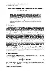
than the average value of normal work months. �(�) ≺ 0 also means that the current time is a depression time or an off season. Accordingly, the manufacturing plant should shorten working hours and reduce the number of employees. Example 1: Consider the system (46) with the system matrices satisfying interval uncertainty (2), where 0.56 1.00 0.60 1.00 , �= , 0.65 0.50 0.70 0.70 0.04 0.06 0.00 0.05 0.07 0.00 �= , �= . 0.00 0.00 0.08 0.00 0.00 0.09

�=

Assume � = 30. Choose the predicted step � = 2 and the initial condition �(�0) = (0.5 0.5)T. By implementing Algorithm 1, we get that Fig. 1 Simulation results of the state �1 under different initial conditions

discrete-time positive linear system, where the aim is to meet the prespecified demand taking into account decisions concerning when to hire and fire, how much inventory to hold, and when to use overtime and undertime. We note that the RMPC could provide a guidance for the aim in [39]. Therefore, we will consider the RMPC of the capacity planning model by slightly modifying the model in [39] as follows: �(� + 1) = �(�)�(�) + �(�)�(�) + �(�)�(�) + �(�)�(�), �(� + 1) = �(�)�(�) + �(�)�(�) + �(�)�(�), (45)

where �(�), �(�) are state variables representing the hours stored in inventory at the beginning of month � and the number of people employed in month �; �(�), �(�), �(�) are decision variables denoting the regular time production hours scheduled in month �, the overtime production hours scheduled in month �, and the number of employees hired at the end of month � for work in month � + 1, respectively; �(�), �(�), �(�) denote the fraction of the total of the hours stored in inventory at the beginning of month �, the fraction of regular time production hours scheduled in month t which are stored in inventory in month � + 1, and the fraction of overtime production hours scheduled in month � which are stored in inventory in month � + 1, respectively; �(�), �(�) are the fraction of employees employed in month � that are retained in month � + 1 and the weight coefficient; �(�), �(�) are the weight coefficients with the relativity between �(�) and �(�). The model (45) can be rewritten as �(� + 1) = �(�)�(�) + �(�)�(�),

(46)

�(�) = (�(�) �(�))T where is the state, �(�) = (�(�) �(�) �(�))T is control input, and the system matrices �(�) =

�(�) �(�)

�(�) , �(�)

�(�) =

�(�) 0

�(�) �(�)

0

.

�=

�=

�

∑ � � �� T)

�=1

( )

( )

�(3) =


−0.0482 , −0.0564 −0.0010 � = −0.0010 , −0.0010

�=

�(1) =

−0.0594 . −0.0574

−0.0492 , −0.0740

0.0016 � = 0.0034 , 0.0074

�(2) =

−0.0492 , −0.0724

Then, the state-feedback control law is −3.9909 −6.0027 �(�) = ��(�) = −3.9909 −5.8703 �(�), −4.8166 −4.6545

(48)

and the lower and upper bounds of the closed-loop system matrix are � + �� =

0.0811 0.2889 , 0.2165 0.0811

� + �� =

0.2009 0.4077 . 0.3147 0.3276 (49)

Finally, the closed-loop system matrix � + �� satisfies � + �� ⪯ � + �� ⪯ � + �� . Choose different initial conditions �(�0) = (0.8 0.4)T, �(�0) = (0.6 0.2)T, and �(�0) = (0.2 0.8)T. Repeating Algorithm 1, we can also get the RMPC for the underlying system, where the corresponding parameters are omitted. Figs. 1 and 2 show the simulation results of the system states �1 and �2. Example 2: Consider the system (46) with the system matrices satisfying polytope uncertainty (4), where 0.56 0.65 0.64 �2 = 0.67

�1 =

(47)

= ��(�T�T� �) +

= ��(�T�T� �) + ⪰ 0,

0.0010 , 0.0010

� = 0.1044,

The equilibrium of the system (46) means that there is no hours stored in inventory at the beginning of month � and no people employed in month �. �(�) ≺ 0 implies that the regular, overtime hours, and the number of employees hired in the month are less

��(�T�T� � +

0.0896 , 0.1172

�

1.00 , 0.50 1.00 , 0.67

∑ ��(�� T)

�=1 �

( )

�=1

0.71 0.77

1.00 , 0.69

( )

∑ (�� ⨂ �)��(� � ) ( )

�3 =

( )

(44)

1795

−5.4092 −4.5758 �(�) = ��(�) = −5.4092 −4.5758 �(�) . −5.4092 −4.5758

(50)

Furthermore (see (51)) Choose different initial conditions �(�0) = (0.8 0.4)T, �(�0) = (0.6 0.2)T, and �(�0) = (0.2 0.8)T. Repeating Algorithm 1, we can also get the RMPC for the underlying system, where the corresponding parameters are omitted. Figs. 3 and 4 show the simulation results of the system states �1 and �2.

5 Conclusions

This paper has solved the RMPC design of uncertain positive systems. First, a performance index with a linear cost function is addressed. Then, by using a linear copositive Lyapunov function associated with linear programming technique, two classes of RMPC control laws are designed for interval uncertain and polytope uncertain positive systems, respectively. A cone invariant

Fig. 2 Simulation results of the state �2 under different initial conditions

�1 + �1� =

0.1273 0.6339 , 0.2714 0.1797

�2 + � 2� =

0.0450 0.4967 , 0.1832 0.2582


0.03 0.05 0.00 0.04 0.07 0.00 , �2 = , 0.00 0.00 0.07 0.00 0.00 0.09 0.06 0.05 0.00 �3 = . 0.00 0.00 0.08

�1 =

Assume � = 30. Choose the predicted step � = 2 and the initial condition �(�0) = (0.5 0.5)T. By implementing Algorithm 1, we get 0.1652 �= , 0.2144 �=

0.0010 , 0.0010

� = 0.1908, �

(3)

−0.1192 �= , −0.1007 −0.0010 � = −0.0010 , −0.0010

�(1) =

−0.1202 = −0.1017

−0.1202 , −0.1017

0.0030 � = 0.0063 , 0.0130

�(2) =

−0.1202 , −0.1017

at the sampling time 0. Thus, the state-feedback control law

0.1150 0.4967 0.3373 0.3239

(51)


set is introduced for positive systems. Several optimisation problems are presented to compute the minimisation bound of the performance index. By induction, it is verified that the present RMPC algorithm is recursively feasible. Finally, the systems considered in the paper are positive and robustly asymptotically stable under the designed control laws.

6 Acknowledgments The authors thank the anonymous reviewers and associate editor for their valuable suggestions and comments which have helped to improve the quality of the paper. This work was supported in part by the National Nature Science Foundation of China (Grant nos. 61503107, 61203123, 61573069), the Zhejiang Provincial Natural Science Foundation of China (Grant no. LY16F030005), and the Open Foundation of First Level Zhejiang Key in Key Discipline of Control Science and Engineering.

7 References [1] [2] [3] [4]

1796

�3 + �3� =

Farina, L., Rinaldi, S.: ‘Positive linear systems: theory and applications’ (Wiley, New York, 2000) Kaczorek, T.: ‘Positive 1D and 2D systems’ (Springer-Verlag, London, 2002) Bru, R., Romero, S., Sanchez, E.: ‘Canonical forms for positive discrete-time linear control systems’, Linear Algebr. Appl., 2000, 310, (1–3), pp. 49–71 Shorten, R., Wirth, F., Leith, D.: ‘A positive systems model of TCP-like congestion control: asymptotic results’, IEEE/ACM Trans. Netw., 2006, 14, (3), pp. 616–629


[5] [6] [7] [8] [9] [10] [11] [12] [13] [14] [15] [16] [17]

[18] [19]

[20] [21]

Liu, X., Wang, L., Yu, W.: ‘Stability analysis for continuous-time positive systems with time-varying delays’, IEEE Trans. Autom. Control, 2011, 55, (4), pp. 1024–1028 Shen, J., Lam, J.: ‘ �1-gain analysis for positive systems with distributed delays’, Automatica, 2014, 50, (1), pp. 175–179 Luenberger, E.: ‘Introduction to dynamic systems: theory, models, and applications’ (Wiley, New York, 1979) Mason, O., Shorten, R.: ‘On linear copositive Lyapunov functions and the stability of switched positive linear systems’, IEEE Trans. Autom. Control, 2007, 52, (7), pp. 1346–1349 Knorn, F., Mason, O., Shorten, R.: ‘On linear co-positive Lyapunov functions for sets of linear positive systems’, Automatica, 2009, 45, (8), pp. 1943–1947 Fornasini, E., Valcher, M.E.: ‘Linear copositive Lyapunov functions for continuous-time positive switched systems’, IEEE Trans. Autom. Control, 2010, 55, (8), pp. 1933–1937 Blanchini, F., Colaneri, P., Valcher, M.E.: ‘Co-positive Lyapunov functions for the stabilization of positive switched systems’, IEEE Trans. Autom. Control, 2012, 57, (12), pp. 3038–3050 Zhao, X., Zhang, L., Shi, P. , et al..: ‘Stability of switched positive linear systems with average dwell time switching’, Automatica, 2012, 48, (6), pp. 1132–1137 Ait Rami, Tadeo, M., F.: ‘Controller synthesis for positive linear systems with bounded controls’, IEEE Trans. Circuits Syst. II Expr. Briefs, 2007, 54, (2), pp. 151–155 Ait Rami, M., Tadeo, F., Benzaouia, A.: ‘Control of constrained positive discrete systems’. Proc. 2007 American Control Conf., Marriott Marquis, New York, USA, 2007, pp. 5851–5856 Ait Rami, M: ‘Solvability of static output-feedback stabilization for LTI positive systems’, Syst. Control Lett., 2011, 60, pp. 704–708 Chen, X., Lam, J., Li, P. et al.: ‘ ℓ1-induced norm and controller synthesis of positive systems’, Automatica, 2013, 49, (5), pp. 1377–1385 Briat, C.: ‘Robust stability and stabilization of uncertain linear positive systems via integral linear constraints: �1- and �∞-gains characterization’, Int. J. Robust Nonlinear Control, 2013, 23, (17), pp. 1932–1954 Zhao, X., Zhang, L., Shi, P.: ‘Stability of a class of switched positive linear time-delay systems’, Int. J. Robust Nonlinear Control, 2013, 23, (5), pp. 578– 589 Xiang, M., Xiang, Z.: ‘Stability, �1-gain and control synthesis for positive switched systems with time-varying delay’, Nonlinear Anal. Hybrid Syst., 2013, 9, pp. 9–17 Lian, J., Liu, J.: ‘New results on stability of switched positive systems: an average dwell-time approach’, IET Control Theory Appl., 2013, 7, (12), pp. 1651–1658 Zhang, J., Han, Z., Zhu, F.: ‘Finite-time control and �1-gain analysis for positive switched systems’, Optim. Control Appl. Meth., 2015, 36, (4), pp. 550–565


[22] [23] [24] [25] [26] [27] [28] [29] [30] [31] [32] [33] [34] [35] [36] [37] [38] [39]

Gao, H., Lam, J., Wang, C. , et al..: ‘Control for stability and positivity: equivalent conditions and computation’, IEEE Trans. Circuits Syst. II Expr. Briefs, 2005, 52, (9), pp. 540–544 Shu, Z., Lam, J., Gao, H., et al..: ‘Positive observers and dynamic outputfeedback controllers for interval positive linear systems’, IEEE Trans. Circuits Syst. I Regul. Pap., 2008, 55, (10), pp. 3209–3222 Kwakernaak, H., Sivan, R.: ‘Linear optimal control systems’ (WileyInterscience, New York, 1972) Hu, S., Zhu, Q.: ‘Stochastic optimal control and analysis of stability of networked control systems with long delay’, Automatica, 2003, 39, (11), pp. 1877–1884 Das, T., Mukherjee, R.: ‘Optimally switched linear systems’, Automatica, 2008, 44, pp. 1437–1441 Basin, M., Rodriguez-Gonzalez, J., Martinez-Zuniga, R.: ‘Optimal control for linear systems with time delay in control input’, J. Franklin Inst., 2004, 341, (3), pp. 267–278 Beauthier, C., Winkin, J.: ‘LQ-optimal control of positive linear systems’, Optim. Control Appl. Methods, 2010, 31, pp. 547–566 Colaneri, P., Middleton, R., Chen, Z. , et al..: ‘Convexity of the cost functional in an optimal control problem for a class of positive switched systems’, Automatica, 2014, 50, pp. 1227–1234 Kothare, M., Balakrishnan, V., Morari, M.: ‘Robust constrained model predictive control using linearm atrix inequalities’, Automatica, 1996, 32, (10), pp. 1361–1379 Diehl, M., Bjornberg, J.: ‘Robust dynamic programming for min-max model predictive control of constrained uncertain systems’, IEEE Trans. Autom. Control, 2004, 49, (12), pp. 2253–2257 Cuzzola, F., Geromel, J., Morari, M.: ‘An improved approach for constrained robust model predictive control’, Automatica, 2002, 38, pp. 1183–1189 Ding, B., Xi, Y., Li, S.: ‘A synthesis approach of on-line constrained robust model predictive control’, Automatica, 2004, 40, pp. 163–167 Li, D., Xi, Y.: ‘The feedback robust MPC for LPV systems with bounded rates of parameter changes’, IEEE Trans. Autom. Control, 2010, 55, (2), pp. 503–507 Hernandez-Vargas, E., Middleton, R., Colaneri, P. et al.: ‘Discrete-time control for switched positive systems with application to mitigating viral escape’, Int. J. Robust Nonlinear Control, 2011, 21, (10), pp. 1093–1111 Gonzaez, A., Roque, A., Garcia-Gonzalez, J.: ‘Modeling and forecasting electricity prices with input/output hidden Markov models’, IEEE Trans. Power Syst., 2005, 20, (1), pp. 13–24 Zijm, W.H.M.: ‘Towards intelligent manufacturing planning and control systems’, OR-Spektrum, 2000, 22, (3), pp. 313–345 Berry, W., Whybark, D., Jacobs, F.: ‘Manufacturing planning and control for supply chain management’ (McGraw-Hill/Irwin, New York, 2005) Caccetta, L., Foulds, L., Rumchev, V.: ‘A positive linear discrete-time model of capacity planning and its controllability properties’, Math. Comput. Model., 2004, 40, (1), pp. 217–226

1797