nyxS. N l. nyxS nyx. Var n n. (6). â« Fade-out. The fade-out transition is that the previous shot disappears gradually and ends at a full frame with a certain color.
Robust Shot Change Detection Models Using Spatial and Temporal Features Yong-Ren Huang*, Hung-Shiang Wang, Chung-Ming Kuo and Chaur-Heh Hsieh Department of Information Engineering I-Shou University, Tashu, 840, Kaohsiung, Taiwan *Department of Information Science Meiho Institute of Technology, Pingtung, Taiwan Abstract—In this paper, we propose various shot change detection models using spatial and temporal features. First, the short-term and long-term variations are discussed for the video shot change. Then, various robust shot change detection models are developed for detecting abrupt and gradual transitions. The residual image, frame difference and the motion compensation are employed in our short-term and long-term algorithms. Finally, Experimental results show that our models for shot change detection are robust compared to conventional algorithms. Key Words — shot change detection, short-term, long-term, abrupt and gradual transitions.
1. INTRODUCTION In substance, shot change is classified into two types, denoted as abrupt and gradual transitions. Abrupt transition is hugely changed between two successive frames which are usually the edge of two shots. These shots contain different content of backgrounds and objects. The spatial features, luminance and color, are immediately changed during these shots. So, the analysis of different frame difference (DFD) will appear a higher peak. Gradual transition is composed of several connective frames with special effects, such as fade-in, fade-out, dissolving and wiping. And there is no obvious peak in the analysis of DFD, because the view of the previous and following shots changes gradually. There are several methods have been proposed for shot change detection. The intensity template matching method is proposed for detecting abrupt shot change[1][2]. The false alarms will appear in these methods because intensity difference magnitude is sensitive to noise, fast object motion, and camera operations. Tonomura [3], Nagasaka and Tanaka [1] proposed the analysis of histogram difference magnitude. These methods may not reflect the difference of content in two successive shots. While the histograms are similar in these shots, it will be failed to detect the change of shots. In block-based methods [4], the local attributes is used for reducing the effect of noise, slow camera and object movement. If there are camera operations or fast objects movement, the false alarm will also appear in this method. Twin-comparison method was proposed for the detection of gradual shot change using two fixed thresholds [5][6][7]. A high threshold is used to detect an abrupt cut. Another lower threshold is employed to identify the candidate frame of gradual shot change. If the accumulated difference between two thresholds, a gradual shot change is detected. In this paper, we propose various new shot change models which are based on short-term and long-term motion compensation. We do not only obtain temporal
features from motion information, but also we can obtain spatial features in residual image. These detection models are developed for detecting the tendencies of shots change, and the threshold decision is avoided. Our proposed methods are represented obviously in section 2. In sub section 2.1, the short-term and long-term variations are discussed. In sub section 2.2, we develop various robust shot change detection models. Then, the experimental results are represented in section 3. Finally, we describe our conclusions in section 4. 2. THE PROPOSED METHODS In this paper, we developed the new shot change models based on motion compensation. Since the human’s eyes are sensitive to brightness; therefore, the motion estimation and motion compensation are only processed in the luminance Y component. The short-term and long-term motion compensation of successive frames is used for detecting the change of shots. The detail algorithms are described in following sub sections. 2.1 Short-Term and Long-Term Variations Generally, lots of shot change detection techniques are only developed in short-term variation under considering two continuous frames. The short-term variation is sensitive to the noise, such as the camera flash or fast object(s) motion. The long-term variation is considered the variation of two frames which stride across several successive frames. If the noise appears, the long-term variation only shows a narrow peak, as shown in Fig.1(a). When a real shot change happens, the short-term variation will appear a narrow peak, and the long-term will show a plateau, represented in Fig.1(b). These results are useful for reducing false alarms caused by noise. (a)
(b)
Short-term
Long-term
Short-term
Long-term
Fig.1 Compared with the noise and cut. (a) Noise in short-term and long-term. (b) Scene change in short-term and long-term.
2.2 Models of various Shot Change types There are two kinds of shot transitions which are abrupt and gradual. The abrupt transition is a huge change between two frames, and the gradual transition which is composed of several frames with some effects, such as fade-in, fade-out, dissolve and wipe. The fade of video sequence is a transition with the first shot gradually disappearing before the second shot gradually appearing. The dissolving is a shot transition with the first shot disappearing while the second shot appearing. And the wiping in a video sequence is a transition with the second shot shifting over the first shot. 2.2.1 Abrupt Shot Change Model We can formulate the shot model S(x,y,n) as follows: S ( x , y , n ) , n < N b S (x , y , n ) = 1 S 2 (x , y , n ) , n ≥ N b
N
2.2.2 Gradual Transition Models There are several categories of video gradual transitions, such fade-in, fade-out, dissolving, wiping. The detail analysis of gradual transitions is described in following. � Fade-in The fade-in transition is beginning at a full frame with a certain color and appearing a new shot gradually. The fade-in edit model can be formulated as follows: (2) T ( x , y , n ) = α (l ) ⋅ C + (1 − α (l ))S 2 ( x , y , n ) where the transition frames N b ≤ n ≤ N e , the transition length 0 ≤ l ≤ (N e − N b = N ) , Nb and Ne are the beginning and ending frames number of the fade-in transition respectively. C is a constant which is a full frame in a certain color, and S2(x,y,n) is the frames of following shot. And α(l) is a decreasing function as follows.
N2
where the Var is variation function. In the form of long-term, because of no obvious motion in the previous shot S1 and the transition frames T(x,y,Nb+l). The long-term variances can be obtained from each two frames difference in the fade-in transition duration, which are decreasing. The long-term variation is developed in Eq.6, and the curve is shown in Fig.2(b). l (6) Varn −1,n (x, y , n ) = ([S1 (x, y , n )] − S2 (x, y , n ) ) 2 N
(a)
(b)
Fig. 2 Variances curve of fade-in model (a)short-term (b) long-term
�
Fade-out The fade-out transition is that the previous shot disappears gradually and ends at a full frame with a certain color. Then the following shot appears suddenly. The fade-out edit model can be formulated in following. (7) T (x , y , n ) = α (l ) ⋅ S 1 (x , y , n ) + (1 − α (l )) ⋅ C where S1(x,y,n) is the previous shot frames. In short-term, the beginning frame of transition duration is similar to S1. In other words, α(l)=α(0)=1 and T(x,y,Nb)=S1(x,y,n). Then, the next frame T(x,y,Nb+1) can be simplified as follows: T (x , y , N b + 1 ) = α (1 ) ⋅ S 1 (x , y , n ) + (1 − α (1 )) ⋅ C (8) N -1 1 = S 1 (x , y , n ) + C N
N
The variances of frames difference are only considered in fade-out transition duration, which are almost a constant (see Fig.3(a)). 1 N −1 Varn +1, n (x, y, n ) = ( S1 ( x, y, n ) + C − S1 (x, y, n ))2 N N 1 = 2 [C − S1 ( x, y, n )]2 N
(9)
In the long-term motion compensation, we also consider the variance of frame difference. The variance of each frame difference in the fade-out transition duration is increasing, which is developed in Eq.10 and shown in Fig.3(b). N − l (10) Var n + l , n (x , y , n ) = ( S 1 (x , y , n ) − S 1 (x , y , n )) 2 N
(3)
In short-term, the beginning frame of transition duration is constant. In other words, α(l)=α(0)=1 and T(x,y,Nb)=C. Then, the next transition frame T(x,y,Nb+1) can be simplified as follows. T (x , y , N b + 1 ) = α (1 ) ⋅ C + (1 − α (1 ))S 2 ( x , y , n ) (4) =
N
(1)
Where S1 and S2 are two continuous shots. And Nb is the cut time. When the position n of frame is less or not less than Nb, the motion compensation can be done between each two continuous frames in shot S1 and S2 individually. Therefore, the short-term variances of residual frames will be almost a constant. While the position n of frame is equal to Nb, the motion compensation will not be done between the frame S1(x,y,Nb-1) and S2(x,y,Nb). So, the short-term variance of residual frame will be very large. In other words, an obvious peak will appear at the beginning of shot change in the time axis. In long-term situation, we define L as a long-term distance of frames. The motion compensation can not be done between the frames in S1 and S2. Therefore, the variation time axis will show continuous L peaks which form a plateau, as shown in Fig.1(b).
N − (N b + l ) N − l α (l ) = e = N e − Nb N
consider the variances of frames difference. And the variances of each frames difference in the fade-in transition duration are almost a constant, which are proved in Eq.5 and shown in Fig.2(a). 1 1 1 Varn−1,n (x, y, n) = ( S2 (x, y, n) − C)2 = [S2 (x, y, n) − C]2 (5)
(a) (b) Fig..3 Variance curve of fade-out model (a)short-term (b) long-term.
N -1 1 S 2 (x , y , n ) + C N N
Because there is no obvious motion between the transition frames T(x,y,Nb+l-1) and T(x,y,Nb+l), we only
�
Dissolving The dissolving transition is that the previous shot
disappears gradually while the following shot appears gradually. The Dissolving edit model can be formulated in following. T (x , y , n ) = α (l )S 1 ( x , y , n ) + (1 − α (l ))S 2 (x , y , n ) (11) In short-term variation, the beginning frame of transition duration is similar to the previous shot S1. So, α(l)=α(0)=1 and T(x,y,Nb)=S1(x,y,n) are established. Then, the next frame T(x,y,Nb+1)can be simplified as follows: (12) T ( x , y , N b + 1 ) = α (1 )S 1 (x , y , n ) + (1 − α (1 ))S 2 (x , y , n ) N − 1 1 = S 1 (x , y , n ) + S N N
2
(x ,
y,n
N
N
N
Case 2: motion compensation between S2 and transition duration Due to gradually appearing the following shot S2, the motion compensation can not be done between S2 and frame T(x,y,Nb+l). Therefore, the variance of frames difference is used to be instead of motion compensation. the variances of frames in the dissolving transition duration are decreasing, which is proved in Eq.15 and shown in Fig.4(b). Accordingly, the motion compensation can be done between T(x,y,Nb+l-1) and T(x,y,Nb+l), so we consider the variance of residual image. The variances of residual Varn+1.n (x, y, n)
= (S1(x, y, n)[u(x − (l − 1)d x ) − u(x − ldx )]
(
(a)
(15)
(b)
Fig. 4 Variance curve of dissolving model (a)short-term (b)long-term.
In long-term, we divided the dissolving transition duration into two cases for discussion. The first one is considering the residual image after motion compensation between the previous shot S1 and transition duration frames. The other is considering frames difference between the second shot S2 and the transition duration frames. We discuss the cases in detail as follows. Case 1: motion compensation between S1 and transition duration Because the previous shot S1 is disappearing gradually, we can do the motion compensation between S1 and transition frame T(x,y,Nb+l). The variances can be obtained from each residual image in the dissolving transition duration are increasing, and we prove in Eq.14 and show in Fig.4(b). Var n + l , n (x , y , n ) = ( S 1 (x , y , n ) (14) l N − l − S 1 (x , y , n ) + S 2 (x , y , n ) ) 2
l N − l − S 1 (x , y , n ) + S 2 (x , y , n ) ) 2 N N
)
Because there is no obvious motion between the transition frames T(x,y,Nb+l-1) and T(x,y,Nb+l), we only consider the variances of frames difference. The variances of the dissolving transition duration are almost a constant proved in Eq.13, as shown in Fig. 4(a). −1 1 (13) Varn +1,n (x, y , n ) = ( S1 (x, y , n ) + S2 (x , y , n ))2 N
Var n + l , n (x , y , n ) = ( S 2 (x , y , n )
(21)
)
− S2 x + x f − dx , y, n [u(x − (l −1)d x ) − u(x − ldx )])2
Due to no obvious change in the transition variances of the short-term residual images, so the curve of short-term variances is flat, but not a peak. In long-term, the compensation can be done between T(x,y,Nb+l-L) and T(x,y,Nb+l). Therefore, we also consider the variances of residual images. The variances of residual images in the wipe transition duration are increasing in the first half and decreasing in the last half. We prove in Eq.22 and show the variation curve in Fig.5(b).
�
Wiping The wiping transition is that the following shot S2 wipes over the previous shot S1. Now, we assume S1 is a still image and S2 is wiping in various angles in the transition duration. From signal viewpoint, wiping edit model can be formulated as follows.
(
)
T (x, y, n ) = S 2 x + x f − l ⋅ d x , y, n [u (x ) − u(x − l ⋅ d x )] + S1 ( x, y, n )[u (x − l ⋅ d x )]
(16)
where dx is the speed of linear wiping, and u(x) is a mask function, shown in Eq.17, Eq.18. w pixels (17) The shifting speed = d x = sec
te − t s
(18)
1 x ≥ 0 u( x) = 0 x < 0
There are several types in the wiping transition, such as left-right wipe-in, top-down wipe-in, bottom-up wipe-in, center-growing and left top-right down wipe-in etc. These wiping types are all similar in the short-term and long-term features. The wiping edit model can be formulated as follows. T ( x, y , tn ) = S 2 ( x + x f − n ⋅ d x , y , tn ) u ( x ) − u ( x − n ⋅ d x ) (19) + S1 ( x, y , tn ) u ( x − n ⋅ d x ) − u ( x − x f )
Where xf is right bound, n is the index of transition frames, dx is the average distance of wiping and tn is time axis of transition. In short-term, the beginning frame of transition duration is similar to S1. In other words, T(x,y,Nb)=S1(x,y,n). Then, the next frame T(x,y,Nb+1) can be simplified as follows.
(
)
T (x , y , N b + 1) = S2 x + x f − 1 ⋅ d x , y , n [u (x ) − u (x − 1 ⋅ d x )]
[
(
+ S1 (x , y , n ) u (x − 1 ⋅ d x ) − u x − x f
)]
(20)
images in the wiping transition duration are almost a constant. It is proved in Eq.21 and shown in Fig.5(a). Varn + l ,n (x, y, n ) = ( S1 (x, y, n )[u(x ) − u(x − ld x )]
(
)
− S2 x + x f − ld x , y, n [u(x ) − u(x − ld x )])2
(a)
(b)
Fig. 5 Variance curve of wiping (a)short-term (b)long-term.
(22)
3. EXPERIMENTAL RESULTS There are ten test fragments of advertisement video which include cut, fade-in, fade-out, dissolving and wiping transitions in our video database, denoted in Table 1. Generally, the length of gradual transitions is about 10 frames in advertisement video sequences. Therefore, we observed a series of the variation between current and successive 15 frames. For reducing the complexity of computation, we employ the Improved Three Steps Searching (ITSS) algorithm for motion estimation. Moreover, the frame size of video is 320x240 pixels. Fig.7 shows the curves of abrupt shot change of NANAKO-1 in short-term and long-term. NANAKO-1 fragment contains 61 frames from 136 to 196 and the cut happens at frame 166. Fig.8 shows the curves of fade-in transition of two NANAKO-1 fragments in short-term and long-term. The fade-in transition is frame 459 to 470. The fragment, Fresh Orange Juice and Beach Section, is processed with fade-out model in short-term and long-term, shown in Fig.9. The fragment is from 182 to 235, and the transition happens from frame 201 to 212. Fig.10 represents the curves of dissolving transition of Melting in short-term and long-term. The first fragment is from frame 56 to 121, and the transition appears from frame 78 to 90. In Fig.11, the curves are the wiping transitions of Swatch-Single Direction in short-term and long-term respectively. The fragment is from frame 56 to 100, and the transition appears from frame 68 to 80. In short-term, the curve is plat. But in long-term, it is a parabola curve that is the same as dissolving. The performance of our methods is shown in Table-2. These experimental results prove that our methods are accurate and robust for detecting shot changes. The performance valuation of the shot change detection is usually expressed by recall and precision. The expressions of recall and precision are defined as follows. Recall =
Nc Nc 100%, Precision = 100% Nc + Nm Nc + N f
where N c is number of correct detection;
gradual transition detection, are matching our algorithms. In wiping transition, we only perform the left-right shifting video sequence. Additionally, the wiping edit model can be extended to detect other kinds of wiping, such as diagonal, circular and so on. 4. CONCLUSIONS In this paper, we developed several shot change detection models based on spatial and temporal features. We employ the residual image, frame difference and motion information for obtaining the variances. The residual and difference information are achieved through the short-term and long-term algorithms. In fact, the spatial and temporal features can be used for detecting cut, fade-in, fade-out, dissolving and wiping. The advantages of our algorithms are that we can classify the changes accurately. The false alarms are avoided, which are caused by camera flash and fast object(s) motion. The experimental results show that our models for shot change detection are robust compared to conventional algorithms. About the high complexity of computation, it is still a challenge in our future works. REFERENCES [1] [2] [3]
[4] [5] [6]
(23)
N m is the number of miss;
[7]
N f is the number of false detection; N c + N m is the number of total true scene changes; N c + N f is the number of total detected;
The experiment results shown above, abrupt and
Nagasaka and Y. Tanaka, “Automatic videos indexing and full-video search for object appearance,” IFIP: Visual Database Systems II, pp 113-127, 1992. H. J. Zhang, A. Kankanhalli, and S. Smoliar, ”Automatic Partitioning of Full Motion Video,” ACM Multimedia Systems, Vol. 1, No. 1, pp.10-28, 1993. Y. Tonomura, “Video handling based on structured information for hypermedia systems,” International Conference on Multimedia Information Systems ’91, 1606, November 1991. R. Kasturi and R. Jain, Dynamic vision, in Computer Vision : Principles, IEEE Computing Society., Los Alamitos, CA, pp. 469-480, 1990. H. J. Zhang, A. Kankanhalli, and S. Smoliar, “Automatic Partitioning of Full-Motion Video,” ACM Multimedia Systems, Vol. 1, No. 1, pp.10-28, 1993. H.B. Lu, Y.J. Zhang, Y.R. Yao, ” Robust gradual scene change detection,” International Conference on Image Processing Proceedings 1999, Vol. 3, 304 –308, 1999. C.L. Huang; B.Y. Liao, ”A robust scene-change detection method for video segmentation,” IEEE Transactions on Circuits and Systems for Video Technology, Vol. 11 Issue: 12, pp. 1281-1288, Dec. 2001.
Table-1 Test video sequences. Sequence Image Abrupt Fade-in Fade-out Dissolve Wipe Length Size 449 320*240 12 0 0 0 0 NANACO-7 901 320*240 12 2 2 2 0 MAYA Artificial 447 320*240 0 0 0 0 8 Wipe Video
Table-2 Recall and precision of test video sequences. Video Abrupt Fade-in Fade-out Dissolve Wipe Recall Precision 12 0 0 0 0 100% 100% NANACO-7 12 2 2 0 94.44% 100% 1 MAYA 0 0 0 0 8 100% 100% Artificial Wipe
Dissolve
Fade-in
Fade-out
Wipe
Fig.6 Types of gradual transition.
Short-term Long-term
4000
4500
3500
4000
3000
3500
2500
3000
2000 1500
2500 2000 1500
1000
1000
500
500 0
0 136
142
148
154
160
166 Fram e
172
178
184
190
Fig.7 Abrupt transition of NANAKO-1 sequence.
Orange Juice and Beach
449
455
461
467 473 Frame
2700 2400
Variance
Variance
2100 1500 1200 900 600 300 0
182
188
194
200
206
212
218
224
230
Frame
6500 6000 5500 5000 4500 4000 3500 3000 2500 2000 1500 1000 500 0
52
58
64
70
76
82
88
94 100 106 112 118 124
Frame
Fig.9 Fade-out transition of Orange Juice and Beach sequence.
Swatch-Single Direction
485
Short-term Long-term
Melting
Short-term
1800
479
Fig.8 Fade-in transition of NANAKO-1 sequence.
Long-term
Variance
Short-term Long-term
NANAKO-1
Variance
Variance
NANAKO-1
short-term long-term
3300 3000 2700 2400 2100 1800 1500 1200 900 600 300 0 56 59 62 65 68 71 74 77 80 83 86 89 92 95 98 Frame
Fig.11 Wiping transition of Swatch-Single Direction sequence.
Fig.10 Dissolving transition of Melting sequence.