Hindawi Wireless Communications and Mobile Computing Volume 2019, Article ID 6592406, 9 pages https://doi.org/10.1155/2019/6592406
Research Article Robust Shrinkage Range Estimation Algorithms Based on Hampel and Skipped Filters Chee-Hyun Park 1 2
1
and Joon-Hyuk Chang
2
Department of Electronics and Computer Engineering, Hanyang University, Seoul 133-791, Republic of Korea Department of Electronic Engineering, Hanyang University, Seoul 133-791, Republic of Korea
Correspondence should be addressed to Joon-Hyuk Chang;
[email protected] Received 28 September 2018; Accepted 18 December 2018; Published 1 January 2019 Guest Editor: Seok-Chul Kwon Copyright © 2019 Chee-Hyun Park and Joon-Hyuk Chang. This is an open access article distributed under the Creative Commons Attribution License, which permits unrestricted use, distribution, and reproduction in any medium, provided the original work is properly cited. Herein, we present robust shrinkage range estimation algorithms for which received signal strength measurements are used to estimate the distance between emitter and sensor. The concepts of robustness for the Hampel filter and skipped filter are combined with shrinkage for the positive blind minimax and Bayes shrinkage estimation. It is demonstrated that the estimation accuracies of the proposed methods are higher than those of the existing median-based shrinkage methods through extensive simulations.
1. Introduction Range estimation is a crucial technique in which the distance between the emitter and sensor is estimated utilizing timeof-arrival (TOA) or received signal strength (RSS) measurements. Distance information is important for range-based source localization utilizing TOA and RSS measurements because distance is used for source localization. Namely, the more accurate is the distance measurement; the better is the localization accuracy. Range estimation problems under lineof-sight (LOS) environments have been studied in previous works [1–5]. In [1], the ad hoc closed-form hybrid TOA/RSS range estimation algorithm is developed. The ad hoc closedform range estimator is superior to the iterative maximum likelihood (ML) method in a certain parameter space. Also, a fusion algorithm is studied for range-based tracking using two independent processing chains for RSS and TOA [2]. In addition, the Cram´er-Rao lower bound (CRLB) for the TOA/RSS-based range estimation is derived in [3]. The RSSbased ranging is famous for its low cost; thus it is more popular than the TOA-based ranging algorithm. In [4], the best unbiased and linear minimum mean square range estimates are studied in the context of RSS-based range estimation. Also, a range estimation method based on the multiplicative distance-correction factor (MDCF) is developed to attenuate
the inaccuracy for the estimated range, where grid based optimization and particle swarm optimization are employed [5]. The shrinkage estimation approach has received attention because it outperforms the ML and least squares (LS) in conditions of small samples or low signal-to-noise ratio (SNR). Although the shrinkage algorithms based on mathematical optimization methods are superior to the blind minimax estimation, we adopt the positive blind minimax (PBM) algorithm in this paper because its computational complexity is much simpler than that of the mathematical optimization-based methods [6, 7]. Also, the Bayes shrinkage (BS) estimation is utilized because PBM and BS estimators are known to outperform the conventional shrinkage estimator [7, 8]. However, some open problems exist and a crucial task among range estimation problems is to determine the distance between the emitter and sensor in LOS/non-line-ofsight (NLOS) mixed situations. For example, the LOS path between the source and sensors may be obstructed under indoor scenarios. Motivated by the above problems, we propose the algorithm combining the shrinkage and robustness. To make the shrinkage estimator robust to outliers, we adopt the Hampel [9–11] and skipped filters [9]. We summarize our main contributions as follows:
2
Wireless Communications and Mobile Computing (i) The variance of the range estimate based on the Hampel filter is found algebraically. (ii) The variance of the range estimate based on the skipped filter is calculated in the analytical form. (iii) We develop the closed-form robust shrinkage range estimation methods based on the Hampel filter/PBM and Hampel filter/BS estimator. (iv) We propose the closed-form robust shrinkage range estimation methods based on the skipped filter/PBM and skipped filter/BS method.
The algorithms that use the Tyler’s estimator for the robust shrinkage estimation of the covariance matrix have been studied [12–15]. But, to the best of our knowledge, the robust shrinkage approaches combined with the Hampel and skipped filters have not been investigated in the existing literatures. Also, note that the proposed methods are the closed-form algorithms. Thus, the complexities of the proposed algorithms are lower than those of the mathematical optimization or iteration-based algorithms. This paper is organized as follows. Section 2 deals with the LOS/NLOS mixed range estimation problem. Section 3 addresses the existing range estimation methods in detail. Section 4 describes the proposed robust shrinkage distance estimation algorithms based on the Hampel filter, skipped filter, PBM, and BS methods. Section 5 evaluates the mean square error (MSE) performances through simulation results. Section 6 presents the conclusion.
2. Problem Formulation The aim of the range estimation method using RSS measurements is to accurately predict the distance between the emitter and sensor so that the error criterion, e.g., the MSE or squared error, is minimized. In the context of LOS/NLOS mixed range estimation, the RSS measurement equation is determined as [16] 𝑃𝑖 = 𝑃𝑜 − 10𝛾log10
𝑑𝑜 + 𝑛𝑖 , 𝑑
𝑖 = 1, 2, . . . , 𝑀
(1)
where 𝑃𝑖 is the ith RSS for the sensor in decibel (dB), 𝑃𝑜 is the signal strength at the reference distance (𝑑𝑜 ), 𝑑𝑜 is set to 1 m for convenience, 𝑑 is the true range (distance) to be estimated, 𝛾 is the path loss exponent, 𝑛𝑖 is distributed by (1 − 𝜖)𝑁(0, 𝜎12 ) + 𝜖𝑁(𝜇2 , 𝜎22 ) with 𝑀 denoting samples in the sensor, and 𝑁(𝜇, 𝜎2 ) is the Gaussian probability density function (PDF) with mean 𝜇 and variance 𝜎2 , respectively [17]. It is assumed that 𝛾 and 𝑃𝑜 are known a priori from the calibration campaign [18, 19]. The measurement error 𝑛𝑖 is the random process that follows a Gaussian distribution with N(0, 𝜎2 ) in conventional LOS situations. However, the noise distribution rarely follows the conventional Gaussian distribution due to multipath effects in indoor and urban regions. Therefore, the noise distribution should be designed as a twomode Gaussian mixture distribution in which the LOS noise component is distributed as 𝑁(0, 𝜎12 ) and the NLOS noise follows 𝑁(𝜇2 , 𝜎22 ). The LOS noise has a probability of 1−𝜖 and
the NLOS noise has a probability of 𝜖. Like previous research for the LOS/NLOS mixture localization, while the statistics of the inlier can be obtained, the mean and variance of the outlier distribution are unavailable. Here, 𝜖 (0 ≤ 𝜖 ≤ 1) is a measure of contamination, which is usually lower than 0.1 [20–22].
3. Review of Conventional Robust Shrinkage Approaches 3.1. ML-Based Shrinkage Range Estimation Algorithm. In the LOS situations, the shrinkage estimator is obtained by multiplying the ML estimator (𝑑̂ML = 𝑑𝑜 10(𝑃−𝑃𝑜 )/10𝛾 = 𝑑 ⋅10𝑛 ) and shrinkage factor (c) [4, 23], where 𝑃 = (∑𝑀 𝑖=1 𝑃𝑖 )/𝑀, 𝑛 = (∑𝑀 𝑛 )/𝑀. The MSE for the shrinkage range estimation 𝑖=1 𝑖 is represented as follows: 𝑇
MSE = 𝐸 [(𝑐 ⋅ 𝑑̂ML − 𝑑) (𝑐 ⋅ 𝑑̂ML − 𝑑)] = 𝐸 [(𝑐 (𝑑 + V) − 𝑑)𝑇 (𝑐 (𝑑 + V) − 𝑑)] = (𝑐 − 1)2 𝑑2 + 𝑐2 𝐸 [V2 ] + 2𝑐 (𝑐 − 1) 𝑑𝐸 [V]
(2)
≃ (𝑐 − 1)2 𝑑2 + 𝑐2 𝐸 [V2 ] ≃ (𝑐 − 1)2 𝑑2 + 𝑐2 var (𝑑̂ML ) where V is the error of the ML estimate (𝑑̂ML ) and 𝐸[V] ≃ 0 by means of the delta method [24]. Then, the shrinkage factor for distance estimation is derived by minimizing the MSE as follows: 𝑐=
2
𝑑2
𝑑2 + var (𝑑̂ML )
≃
(𝑑̂ML ) 2
(𝑑̂ML ) + var (𝑑̂ML )
.
(3)
The shrinkage range estimator is obtained as follows: 𝑏=
(𝑑̂ML )
2
2 (𝑑̂ML ) + var (𝑑̂ML )
⋅ 𝑑̂ML .
(4)
Although var(𝑑̂ML ) can be calculated analytically, 𝑑̂ML is linearized to apply the shrinkage algorithm (see (2)). For this, the ML range estimator is linearized for E[𝑛] using the Taylorseries as follows: ln 10 𝑑̂ML ≃ 𝑑 ⋅ {10𝐸[𝑛]/10𝛾 + 10𝐸[𝑛]/10𝛾 (𝑛 − 𝐸 [𝑛])} 10𝛾 ln 10 ) 𝑑 ⋅ 𝑛. =𝑑+( 10𝛾
(5)
Then, var{𝑑̂ML } ≃ 𝑑2 ((ln 10)/10𝛾)2 var{𝑃}. Because 𝑑 is an unknown true value to be estimated, the variance of 𝑑̂ML can be approximated as {𝑑̂ML }2 ((ln 10)/10𝛾)2 (𝜎2 /𝑀), where 𝜎2 is the variance per sample. It should be noticed that the approximated variance of 𝑑̂ML is different from the true
Wireless Communications and Mobile Computing
3
variance of 𝑑̂ML as can be seen from our simulation results. Furthermore, the conventional shrinkage estimator can be improved in two ways: the PBM algorithm and BS method. Finally, the PBM estimator is represented as follows [7]: 𝑏PBM = 𝛼PBM ⋅ 𝑑̂ML + (1 − 𝛼PBM ) 𝑑∗ ̂ML 2
̂ML
̂ML 2
(6) ̂ML
where 𝛼PBM = [(𝑑 ) − var(𝑑 )]+ /([(𝑑 ) − var(𝑑 )]+ + var(𝑑̂ML )), 𝑑∗ is the prior point guess value to be determined empirically, and (⋅)+ denotes the max(0, ⋅). Also, the BS estimator is obtained in the following [8]: 𝑏BS = 𝛼BS ⋅ 𝑑̂ML + (1 − 𝛼BS ) 𝑑∗ .
(7)
where 𝛼BS = (𝑑̂ML − 𝑑∗ )2 /((𝑑̂ML − 𝑑∗ )2 + var(𝑑̂ML )). When the prior value, 𝑑∗ , is properly selected, the MSE performance of the BS method is superior to that of the existing shrinkage algorithm. 3.2. Median- (Med-) Based Robust Shrinkage Range Estimation Algorithm. The ML-based range estimator is an optimal estimator in LOS environments; however it becomes much inaccurate when there are outliers among samples. To circumvent this problem, the median-based range estimator can be utilized because it is insensitive to outliers when the contamination ratio is less than 50%. In this case, the median-based range estimator can be represented as ̃ 𝑑̂Med = 𝑑𝑜 10(𝑃−𝑃𝑜 )/10𝛾 , where 𝑃̃ = median{𝑃1 , . . . , 𝑃𝑀 }. Then, in the same manner as the ML-based range estimator, the variance of the median-based robust range algorithm ̃ ≃ (var[𝑑̂Med ]) can be obtained as 𝑑2 ((ln 10)/10𝛾)2 var{𝑃} {𝑑̂Med }2 ((ln 10)/10𝛾)2 (𝜎2 /𝑀)(𝜋/2). Note that, in the derivation of variance of the median-based robust range estimation method, the constant 𝜋/2 is multiplied because the variance of the sample median is asymptotically 𝜋/2 times larger than that of the sample mean in the LOS situation [25]. Also, the median-based shrinkage range estimator can be categorized into the median-based PBM (Med/PBM) and median-based Bayesian shrinkage (Med/BS) estimator. The Med/PBM and Med/BS estimators are represented as follows: 𝑏Med/PBM = 𝛼Med/PBM ⋅ 𝑑̂Med + (1 − 𝛼Med/PBM ) 𝑑∗ 𝑏Med/BS = 𝛼Med/BS ⋅ 𝑑̂Med + (1 − 𝛼Med/BS ) 𝑑∗
(8)
where 𝛼Med/PBM = [(𝑑̂Med )2 − var(𝑑̂Med )]+ /([(𝑑̂Med )2 − var(𝑑̂Med )]+ +var(𝑑̂Med )) and 𝛼Med/BS = (𝑑̂Med −𝑑∗ )2 /((𝑑̂Med − 𝑑∗ )2 + var(𝑑̂Med )).
3.3. Hampel Filter. The version considered, herein, represents a moving-window implementation of the Hampel filter as in [9–11], an outlier detection procedure based on the median and median absolute deviation (MAD) scale estimator. Specifically, this filter’s response is given by {𝑃𝑖 , 𝑃𝑖 − 𝑚 < 𝑡𝐷, 𝑦𝑖 = { (9) 𝑚, 𝑃𝑖 − 𝑚 > 𝑡𝐷 { where 𝑚 is the median value from the moving data window and 𝐷 is the MAD scale estimate of the sensor, defined as 𝐷 = 1.4826 × median|𝑃1:𝑀 − 𝑚|. Namely, the sensors are categorized into the LOS sensor set and LOS/NLOS mixture sensor set with the use of (9). If the entire elements of the sensor meet the first condition of (9), it is predicted as an LOS sensor. If at least one sample satisfies the second condition of (9), the corresponding sensor is regarded as an LOS/NLOS mixture sensor. The factor 1.4826 allows the MAD scale to produce an unbiased estimate of the standard deviation for Gaussian data. Also, 𝑃1:𝑀 is the RSS from the first to the Mth in the sensor and the parameter 𝑡 is selected empirically. When 𝑡 = 0, the Hampel filter is reduced to the standard median filter. The Hampel filter suffers from implosion, which means more than 50% of data values are identical, i.e., 𝐷 = 0, implying that 𝑦𝑖 = 𝑚 irrespective of the constant 𝑡. 3.4. Skipped Filter [9]. In the Hampel filter of the previous section, when the absolute value of the difference between the sample and median is larger than the threshold, the sample median is substituted for the corresponding sample. In contrast, in the skipped filter, when the sample is predicted as an outlier, the corresponding sample is removed from the sample set of the sensor. Because the contamination ratio (the percentage of outliers in the sample set) is usually smaller than 10% [20–22], the probability that the filtered samples are depleted is much small.
4. Proposed Robust Shrinkage Range Estimation Method Below, we explain in detail the proposed Hampel filter-based, skipped filter-based shrinkage range estimation algorithms. 4.1. Hampel Filter/PBM and Hampel Filter/BS-Based Range Estimation Algorithms. In this subsection, the Hampel filterbased shrinkage range estimation algorithms are described in detail. The filtered data, 𝑦1:𝑀 , are averaged using the sample mean, i.e., 𝑃ℎ,𝑓 = (∑𝑀 𝑖=1 𝑦𝑖 )/𝑀. Then, the variance of the statistic 𝑃ℎ,𝑓 is found as follows:
var [𝑃ℎ,𝑓 ] = =
(var [one inlier (𝑦𝑞 )] × number of inliers + var [median for 𝑦𝑖 (𝑖 = 1, . . . , 𝑀)] × number of outliers) 𝑀2 𝑆/𝑄 × 𝑄 + 𝜋/2 × 𝑆/𝑄2 × 𝑅 𝑆 + 𝜋/2 × 𝑆/𝑄2 × 𝑅 = 𝑀2 𝑀2
(10)
4
Wireless Communications and Mobile Computing
where 𝑆 = ∑𝑞 (𝑦𝑞 − 𝑚)2 , 𝑞’s are the sample indices determined as inliers in the LOS/NLOS mixture state, and 𝑄 is the number of samples predicted as inliers with the use of (9). Also, 𝑅 is the number of samples determined as outliers and 𝑀 = (𝑄 + R) is the total number of samples in the sensor. In the numerator of the second equation of (10), the constant 𝜋/2 is multiplied by the variance of the sample mean [25] since the variance of the sample median is asymptotically 𝜋/2 times larger than that of the sample mean in the LOS situation. Furthermore, we do not consider the implosion because it rarely occurs. Then, the variance of the Hampel filter-based range estimator is obtained as var{𝑑̂Ham } ≃ {𝑑̂Ham }2 ((ln 10)/10𝛾)2 ⋅ var[𝑃ℎ,𝑓 ], where 𝑑̂Ham = ℎ,𝑓 𝑑𝑜 10(𝑃 −𝑃𝑜 )/10𝛾 . Additionally, the robust shrinkage range estimator based on the Hampel filter and PBM estimator is obtained as follows: 𝑏Ham/PBM = 𝛼Ham/PBM ⋅ 𝑑̂Ham + (1 − 𝛼Ham/PBM ) 𝑑∗
(11)
where 𝛼Ham/PBM = ((𝑑̂Ham )2 − var(𝑑̂Ham ))+ /(((𝑑̂Ham )2 − var(𝑑̂Ham ))+ + var(𝑑̂Ham )). Furthermore, the robust shrinkage range estimator based on the Hampel filter and BS method is found as 𝑏Ham/BS = 𝛼Ham/BS ⋅ 𝑑̂Ham + (1 − 𝛼Ham/BS ) 𝑑∗
(12)
where 𝛼Ham/BS = (𝑑̂Ham − 𝑑∗ )2 /((𝑑̂Ham − 𝑑∗ )2 + var(𝑑̂Ham )). 4.2. Skipped Filter/PBM and Skipped Filter/BS-Based Range Estimation Methods. In the same manner as the Hampel filter-based shrinkage range estimation method, the filtered data, 𝑦𝑞 , are averaged using the sample mean, i.e., 𝑃𝑠,𝑓 = ∑𝑞 (𝑦𝑞 /𝑄). The variance of the statistic 𝑃𝑠,𝑓 is calculated in the following: var [𝑃𝑠,𝑓 ] = =
var [one inlier (𝑦𝑞 )] × number of inliers 𝑄2
(13)
𝑆/𝑄 × 𝑄 𝑆 = 2. 2 𝑄 𝑄
Then, the variance of the skipped filter-based range estimator is obtained as var{𝑑̂Sk } ≃ {𝑑̂Sk }2 ((ln 10)/10𝛾)2 ⋅ var[𝑃𝑠,𝑓 ], 𝑠,𝑓 where 𝑑̂Sk = 𝑑𝑜 10(𝑃 −𝑃𝑜 )/10𝛾 . Additionally, the robust shrinkage range estimator based on the skipped filter and PBM method is obtained as follows: 𝑏Sk/PBM = 𝛼Sk/PBM ⋅ 𝑑̂Sk + (1 − 𝛼Sk/PBM ) 𝑑∗
(14)
where 𝛼Sk/PBM = ((𝑑̂Sk )2 − var(𝑑̂Sk ))+ /(((𝑑̂Sk )2 − var(𝑑̂Sk ))+ + var(𝑑̂Sk )). Indeed, the robust shrinkage range estimator based on the skipped filter and BS method is obtained as follows: 𝑏Sk/BS = 𝛼Sk/BS ⋅ 𝑑̂Sk + (1 − 𝛼Sk/BS ) 𝑑∗ where 𝛼Sk/BS = (𝑑̂Sk − 𝑑∗ )2 /((𝑑̂Sk − 𝑑∗ )2 + var(𝑑̂Sk )).
(15)
Table 1: Simulation settings. Distance (d) Parameter (d∗ ) Parameter (t) Number of Monte-Carlo simulation Number of sensors Path loss exponent (𝛾) 𝑃𝑜 𝑑𝑜 Directivity of source
5m 10 1.5 1000 1 3 5 dB 1m omnidirection
Table 2: List of abbreviations. TOA RSS LOS ML CRLB MDCF LS SNR PBM BS NLOS dB PDF MSE Med/PBM Ham/BS SK/PBM
Time of Arrival Received Signal Strength Line of sight Maximum Likelihood Cram´er-Rao lower bound multiplicative distance-correction factor Least Squares Signal-to-noise ratio positive blind minimax Bayes shrinkage Non-line-of-sight decibel Probability density function Mean square error Median/Positive blind minimax Hampel filter/Bayes shrinkage Skipped filter/Positive blind minimax
Furthermore, the distance can be also estimated in the energy-based acoustic ranging problem [26, 27]. Unlike the RSS-based ranging algorithm, the reference signal power is not known in the energy-based ranging method. Therefore, the distance cannot be estimated directly from the measurement equation. In this case, the range can be estimated sequentially, i.e., the source location is firstly estimated using the energy minimization-based localization algorithm [27] (the robust version of the measurement is used in the localization algorithm), then the distance is obtained from the estimated position. The shrinkage factor can be found using the estimated source coordinates and delta method. The difference between the shrinkage factor in the LOS situation and that of LOS/NLOS mixture environment lies in that the position estimate using the robust algorithm is utilized under the LOS/NLOS mixed situation. The details for the algorithm and performance evaluation remain as future works.
5. Simulation Results We compare the performance of the proposed LOS/NLOS mixed range estimation methods with that of the medianbased shrinkage range estimator in this section. The simulation setting is provided in Table 1. Table 2 explains the
Wireless Communications and Mobile Computing
5 5
5
0
−5
MSE Average (dB)
MSE Average (dB)
0
−10 −15
−10
−15
−20 −25
−5
1
2
3
4
5 6 Distance (m)
7
8
9
10
−20
1
2
3
4
5 6 Distance (m)
7
8
9
10
Med Med/PBM Ham/BS Sk/PBM Med/BS Ham/PBM Sk/BS
Med Med/PBM Ham/BS Sk/PBM Med/BS Ham/PBM Sk/BS
(b) 𝜖: 30%, 𝜎1 : √10 m, 𝜇2 : 4 m, and 𝜎2 : 100 m
(a) Contamination ratio (𝜖): 20%, the bias of NLOS noise (𝜇2 ): 4 m, standard deviation of LOS noise (𝜎1 ): √10 m, and standard deviation of NLOS noise (𝜎2 ): 100 m
Figure 1: MSE averages of the range estimation algorithms as a function of the distance.
15
abbreviations used in this paper. The MSE average is defined as follows: 1000
10
2
(16)
̂ is the estimated range from the point target to the where 𝑑(𝑘) sensor in the kth range set and 𝑑 denotes the true range to be estimated. Figure 1 is the distance versus MSE averages. As the distance increased, the MSE average increased and the MSE averages of the proposed methods were lower than those of the other methods. Figure 2 is the MSE averages versus the standard deviation of inliers. The MSE averages of the proposed methods were lower than those of the other existing methods based on the median in Figure 2. The performances of all robust methods deteriorated as the standard deviation of LOS error was increased. Figure 3 shows the MSE averages as a function of standard deviation of NLOS noise. The MSE averages for the proposed robust shrinkage range estimation methods were lower than those of the other methods. The localization performances of the proposed and median-based existing algorithms were not affected by the NLOS noise because the Hampel and skipped filters are insensitive to the adverse effects of outliers. Figure 4 shows the MSE averages versus the bias. The MSE averages of all methods were nearly constant as the bias
5 MSE Average (dB)
MSE average =
̂ ∑1000 𝑘=1 (𝑑 (𝑘) − 𝑑)
0 −5 −10 −15 −20
0
5
10 15 Variance of LOS Noise (dB)
20
25
Med Med/PBM Ham/BS Sk/PBM Med/BS Ham/PBM Sk/BS
Figure 2: MSE averages of the range estimation algorithms as a function of variance of LOS noise (bias of NLOS noise (𝜇2 ): 4 m, contamination ratio: 30%, and standard deviation of NLOS noise (𝜎2 ): 100 m).
6
Wireless Communications and Mobile Computing −2.5
−3
−3
MSE Average (dB)
MSE Average (dB)
−3.5
−4
−4.5
−3.5
−4
−4.5 −5
−5.5
−5
70
80 90 100 110 120 Standard Deviation of NLOS Noise (m)
130
Med Med/PBM Ham/BS Sk/PBM Med/BS Ham/PBM Sk/BS
−5.5 0
2
4
6
8
10
Bias (m) Med Med/PBM Ham/BS Sk/PBM Med/BS Ham/PBM Sk/BS
Figure 3: Comparison of MSE averages of the proposed estimators with that of the existing methods (contamination ratio (𝜖): 30%, the bias of NLOS noise (𝜇2 ): 4 m, and standard deviation of LOS noise (𝜎1 ): √10 m).
Figure 4: MSE averages of the range estimation algorithms as a function of bias (contamination ratio: 30%, standard deviation of LOS noise (𝜎1 ): √10 m, and standard deviation of NLOS noise (𝜎2 ): 100 m).
varied and the proposed methods outperformed the other existing algorithms. Namely, the estimation performances of the proposed range estimation algorithms are not affected by the bias because the Hampel and skipped filters are robust to the outliers. Figure 5 shows the variation of the MSE averages with respect to the parameter 𝑡 in (9). The MSE averages of the proposed algorithms, i.e., the Hampel and skipped filter-based methods, were much affected by the selection of parameter 𝑡, but those of the median-based methods were nearly constant and the MSE average of the proposed algorithms was minimal at 𝑡 = 1.5. The MSE averages of the proposed methods are sensitive to the parameter 𝑡 because 𝑃ℎ,𝑓 and 𝑃𝑠,𝑓 are dependent on the value of 𝑡. Figure 6 is the sample size versus the MSE averages. Again, the proposed range estimation methods outperformed the other methods, as shown in Figure 6 and the MSE averages decreased as the sample size increased. Figure 7 shows the variation of the MSE averages with respect to the contamination ratio (𝜖). When the contamination ratio was lower than 50%, the MSE averages of all algorithms increased slightly as the contamination ratio increased. However, when the contamination ratio became larger than 50%, the MSE averages of the existing range estimation methods were significantly increased. Meanwhile, those of the proposed
methods were slightly incremented. Figure 8 shows the true and approximated variances of the ML range estimator. The true variance and approximated variance using the Taylorseries were nearly the same when the standard deviation of LOS noise was √10 m. However, the approximated variance diverged from the true variance when the standard deviation of LOS noise increased to 17 m because the Taylor-series was adopted. Thus, the approximated variance should be utilized to apply the shrinkage estimator effectively.
6. Conclusions The robust shrinkage range estimation methods were developed utilizing the Hampel filter, skipped filter, PBM, and BS estimators. Namely, the concepts of robustness for the Hampel and skipped filters and shrinkage for the PBM and BS estimators were mixed. The MSE performances of the proposed robust shrinkage methods were superior to those of the existing median-based shrinkage algorithms in the various simulation environments. Note that the MSE performances of the proposed methods were more robust, even in the regimes where 𝜖 ≥ 0.5, than those of the median-based shrinkage algorithms. Also, the proposed algorithms were developed in closed-form; thus, the computational complexities would be lower than those of the iteration methods.
Wireless Communications and Mobile Computing
7
−1.5
−3
−2
−4
MSE Average (dB)
MSE Average (dB)
−2.5 −3 −3.5
−5 −6 −7 −8
−4 −9 −4.5 −10 −5 −5.5 0.5
10
15
20
25
Sample Size
1
1.5
2
2.5
3
3.5
Med Med/PBM Ham/BS Sk/PBM Med/BS Ham/PBM Sk/BS
4
t Med Med/PBM Ham/BS Sk/PBM Med/BS Ham/PBM Sk/BS
Figure 6: MSE averages of the range estimation algorithms as a function of sample size (contamination ratio: 30%, standard deviation of LOS noise (𝜎1 ): √10 m, and standard deviation of NLOS noise (𝜎2 ): 100 m.
Figure 5: MSE averages of the range estimation algorithms as a function of parameter (t) (bias of NLOS noise (𝜇2 ): 4 m, contamination ratio: 30%, standard deviation of LOS noise (𝜎1 ): √10 m, and standard deviation of NLOS noise (𝜎2 ): 100 m).
70 60
The datasets generated during and/or analysed during the current study are not publicly available due to the fact that ftp is not available but are available from the corresponding author upon reasonable request.
MSE Average (dB)
50
Data Availability
40 30 20 10
Conflicts of Interest The authors declare that they have no conflicts of interest.
0 −10 0.1
0.2
Authors’ Contributions In this research paper, Chee-Hyun Park proposed a robust shrinkage distance estimation algorithm. Joon-Hyuk Chang carried out the correspondence of the paper.
Acknowledgments This work was supported by Projects for Research and Development of Police Science and Technology under Center for Research and Development of Police Science and Technology and Korean National Police Agency funded by the Ministry of Science and ICT (PA-J000001-2017-101) and was supported by the National Research Foundation of Korea
0.3 0.4 0.5 0.6 Contamination Ratio ()
0.7
0.8
Med Med/PBM Ham/BS Sk/PBM Med/BS Ham/PBM Sk/BS
Figure 7: Comparison of MSE averages of the proposed estimators as a contamination ratio.
(NRF) grant funded by the Korea Government (MOE) (no. 201800000000513).
8
Wireless Communications and Mobile Computing 0.6
25
20 Variance of ML Estimator
Variance of ML Estimator
0.5 0.4 0.3 0.2
10
5
0.1 0
15
1
2
3
4
5 6 Distance (m)
7
8
9
10
True Variance Approximated Variance (a) Standard deviation of LOS noise (𝜎1 ): √10 m
0
1
2
3
4
5 6 Distance (m)
7
8
9
10
True Variance Approximated Variance (b) Standard deviation of LOS noise (𝜎1 ): 17 m
Figure 8: Comparison of true and approximated variances of the ML estimator as a function of distance.
References [1] A. Coluccia and A. Fascista, “On the Hybrid TOA/RSS Range Estimation in Wireless Sensor Networks,” IEEE Transactions on Wireless Communications, vol. 17, no. 1, pp. 216–218, 2018. [2] D. Macii, A. Colombo, P. Pivato, and D. Fontanelli, “A data fusion technique for wireless ranging performance improvement,” IEEE Transactions on Instrumentation and Measurement, vol. 42, no. 8, pp. 1905–1915, 1994. [3] A. Catovic and Z. Sahinoglu, “The Cramer-Rao bounds of hybrid TOA/RSS and TDOA/RSS location estimation schemes,” IEEE Communications Letters, vol. 8, no. 10, pp. 626–628, 2004. [4] S. D. Chitte, S. Dasgupta, and Z. Ding, “Distance estimation from received signal strength under log-normal shadowing: Bias and variance,” IEEE Signal Processing Letters, vol. 16, no. 3, pp. 216–218, 2009. [5] L. Gui, M. Yang, P. Fang, and S. Yang, “RSS-based indoor localisation using MDCF,” IET Wireless Sensor Systems, vol. 7, no. 4, pp. 98–104, 2017. ´ [6] Y. Eldar, “Uniformly Improving the CramEr-Rao Bound and Maximum-Likelihood Estimation,” IEEE Transactions on Signal Processing, vol. 54, no. 8, pp. 2943–2956, 2006. [7] Z. Ben-Haim and Y. C. Eldar, “Blind minimax estimation,” Institute of Electrical and Electronics Engineers Transactions on Information Theory, vol. 53, no. 9, pp. 3145–3157, 2007. [8] L. Li, “Bayesian Shrinkage Estimation in Exponential Distribution Based on Record Values,” in Proceedings of the 2011 International Conference on Computational and Information Sciences (ICCIS), pp. 1159–1162, Chengdu, China, October 2011. [9] R. R. Wilkox, Introduction to robust estimation and hypothesis testing, Academic Press, 3rd edition, 2012. [10] R. K. Pearson, Y. Neuvo, J. Astola, and M. Gabbouj, “Generalized Hampel Filters,” EURASIP Journal on Advances in Signal Processing, pp. 1–18, 2016. [11] F. R. Hampel, “The breakdown points of the mean combined with some rejection rules,” Technometrics, vol. 27, no. 2, pp. 95– 107, 1985.
[12] D. E. Tyler, “A distribution-free 𝑀-estimator of multivariate scatter,” The Annals of Statistics, vol. 15, no. 1, pp. 234–251, 1987. [13] F. Pascal, Y. Chitour, J.-P. Ovarlez, P. Forster, and P. Larzabal, “Covariance structure maximum-likelihood estimates in compound Gaussian noise: existence and algorithm analysis,” IEEE Transactions on Signal Processing, vol. 56, no. 1, pp. 34–48, 2008. [14] Y. I. Abramovich and N. K. Spencer, “Diagonally loaded normalised sample matrix inversion (LNSMI) for outlier-resistant adaptive filtering,” in Proceedings of the 2007 IEEE International Conference on Acoustics, Speech and Signal Processing, ICASSP ’07, pp. III1105–III1108, USA, April 2007. [15] Y. Chen, A. Wiesel, and I. Hero, “Robust shrinkage estimation of high-dimensional covariance matrices,” IEEE Transactions on Signal Processing, vol. 59, no. 9, pp. 4097–4107, 2011. [16] T. S. Rappaport, Wireless Communications: Principles and Practice, Prentice Hall, 2nd edition, 2002. [17] F. Yin, C. Fritsche, F. Gustafsson, and A. M. Zoubir, “EMand JMAP-ML based joint estimation algorithms for robust wireless geolocation in mixed LOS/NLOS environments,” IEEE Transactions on Signal Processing, vol. 62, no. 1, pp. 168–182, 2014. [18] N. Patwari, J. N. Ash, S. Kyperountas, A. O. Hero III, R. L. Moses, and N. S. Correal, “Locating the nodes: cooperative localization in wireless sensor networks,” IEEE Signal Processing Magazine, vol. 22, no. 4, pp. 54–69, 2005. [19] P. Tarrio, A. M. Bernardos, J. A. Besada, and J. R. Casar, “A new positioning technique for RSS-Based localization based on a weighted least squares estimator,” in Proceedings of the 2008 IEEE International Symposium on Wireless Communication Systems, pp. 633–637, Reykjavik, Iceland, October 2008. [20] F. Yin, C. Fritsche, F. Gustafsson, and A. M. Zoubir, “TOAbased robust wireless geolocation and cram´er-rao lower bound analysis in harsh LOS/NLOS environments,” IEEE Transactions on Signal Processing, vol. 61, no. 9, pp. 2243–2255, 2013. [21] F. Gustafsson and F. Gunnarsson, “Mobile positioning using wireless networks: possibilities and fundamental limitations
Wireless Communications and Mobile Computing
[22]
[23]
[24] [25] [26]
[27]
based on available wireless network measurements,” IEEE Signal Processing Magazine, vol. 22, no. 4, pp. 41–53, 2005. U. Hammes, E. Wolsztynski, and A. M. Zoubir, “Robust tracking and geolocation for wireless networks in NLOS environments,” IEEE Journal of Selected Topics in Signal Processing, vol. 3, no. 5, pp. 889–901, 2009. C.-H. Park and J.-H. Chang, “Shrinkage estimation-based source localization with minimum mean squared error criterion and minimum bias criterion,” Digital Signal Processing, vol. 29, pp. 100–106, 2014. G. Casella and R. L. Berger, Statistical Inference, Cengage Learning, 2nd edition, 2001. P. J. Rousseeuw and A. M. Leroy, Robust Regression and Outlier Detection, John Wiley & Sons, 1987. Li and Y. H. Hu, “Energy-based collaborative source localization using acoustic microsensor array,” EURASIP Journal on Advances in Signal Processing, vol. 89, pp. 1–11, 2016. K. C. Ho and M. Sun, “An accurate algebraic closed-form solution for energy-based source localization,” IEEE Transactions on Audio, Speech and Language Processing, vol. 15, no. 8, pp. 2542– 2550, 2007.
9
International Journal of
Advances in
Rotating Machinery
Engineering Journal of
Hindawi www.hindawi.com
Volume 2018
The Scientific World Journal Hindawi Publishing Corporation http://www.hindawi.com www.hindawi.com
Volume 2018 2013
Multimedia
Journal of
Sensors Hindawi www.hindawi.com
Volume 2018
Hindawi www.hindawi.com
Volume 2018
Hindawi www.hindawi.com
Volume 2018
Journal of
Control Science and Engineering
Advances in
Civil Engineering Hindawi www.hindawi.com
Hindawi www.hindawi.com
Volume 2018
Volume 2018
Submit your manuscripts at www.hindawi.com Journal of
Journal of
Electrical and Computer Engineering
Robotics Hindawi www.hindawi.com
Hindawi www.hindawi.com
Volume 2018
Volume 2018
VLSI Design Advances in OptoElectronics International Journal of
Navigation and Observation Hindawi www.hindawi.com
Volume 2018
Hindawi www.hindawi.com
Hindawi www.hindawi.com
Chemical Engineering Hindawi www.hindawi.com
Volume 2018
Volume 2018
Active and Passive Electronic Components
Antennas and Propagation Hindawi www.hindawi.com
Aerospace Engineering
Hindawi www.hindawi.com
Volume 2018
Hindawi www.hindawi.com
Volume 2018
Volume 2018
International Journal of
International Journal of
International Journal of
Modelling & Simulation in Engineering
Volume 2018
Hindawi www.hindawi.com
Volume 2018
Shock and Vibration Hindawi www.hindawi.com
Volume 2018
Advances in
Acoustics and Vibration Hindawi www.hindawi.com
Volume 2018