ROBUST ZEBRA-CROSSING DETECTION USING BIPOLARITY AND PROJECTIVE INVARIANT Mohammad Shorif Uddin and Tadayoshi Shioyama Department of Mechanical and System Engineering Kyoto Institute of Technology, Sakyo-ku, Kyoto 606-8585, Japan E-mail:
[email protected] ABSTRACT Crossing roads is a great challenge for visually impaired people. A robust technique for detection of zebra crossings is described. This is achieved through bipolaritybased segmentation and projective invariant-based recognition. The technique shows good performances under various illuminations such as sunny, cloudy and rainy situations in the day time and also evening and night environments.
ing the vanishing point constraint. But, a thorough evaluation of this technique is not yet performed and it works slow and is far from real time. On the other hand, the present method works very fast. To confirm the robustness of the proposed method, experiment is performed using real road scenes with and without crossings under various illumination conditions such as sunny, cloudy and rainy situations in the day time and also evening and night environments.
1. INTRODUCTION
2. DETECTION PRINCIPLE
Independent walk is the main barrier for the visually impaired people. Usually, they use a white cane. The range of detection of special patterns or obstacles using a cane is very narrow. To improve the versatility of the white cane, various electronic devices [1] have been developed. But, these devices are unable to assist them in safely crossing a road. Some traffic lights have beepers, which prompt the visually impaired to cross the road, when it is safe to do so. However, such equipment is not available at every crossing; perhaps, it would take too long for such equipment to be installed and maintained at every crossing. Blind people obviously can not see, but can hear. The principal objective of this research is to develop a computer vision-based wearable device that uses vocal commands to allow blind people to cross roads with total safety. For a safe road crossing, at first a blind person needs the information about the location of a crossing i.e. whether his frontal area is a crossing or not, then an idea about its length and the state of traffic lights. We have already developed a crossing length measurement technique [2] assuming that the image contains a crossing. Therefore, crossing location detection becomes a prerequisite. Recently, we reported a computer vision-based zebra crossing detection system [3]. lighting environment affects the performance of any computer vision application. However, in that paper we did not investigate the lighting effects. This paper tries to fill this gap. From the view point of a computer vision-based zebra crossing detection, Stephen Se [4] proposed a technique by grouping lines and checking for concurrency us-
A zebra crossing is characterized by evenly spaced white stripes on a usual black road surface. In Japan, the width of each white or black stripe is 45 cm. Some experimental images of real road scenes are shown in Figs. 1 and 2 . The size of images is (width × height) = (640 × 480) pixels. The crossing pattern can be treated as a bipolar region. The proposed technique includes four major steps. To cope with the various lighting situations, first, we use histogram equalization if the average intensity of the image is less than a threshold. Second, we extract the candidate crossing area based on bipolarity feature. Then checking the candidate area for the appropriateness of its position in the image as well as crossing direction, as the technique is searching for a frontal crossing. Third, we extract the feature points on the central vertical line of the binarized candidate area. Fourth, taking the final decision of a crossing or not a crossing using projective invariant. As bipolarity and projective invariant features are used as the main tools in the proposed algorithm, we describe briefly these two in the following subsections.
Thanks to the Japan Society for the Promotion of Science for the support under Grants-in-Aid for Scientific Research (No. 16500110 and No. 03232).
µi =
0-7803-9243-4/05/$20.00 ©2005 IEEE
571
2.1. Bipolarity We denote the intensity distribution of an image block as p0 (x). If the block contains only black and white pixels, then p0 (x) can be written as p0 (x) = α p1 (x) + (1 − α )p2 (x), where 0 ≤ α ≤ 1, p1 (x) is the intensity distribution of black pixels and p2 (x) is the intensity distribution of white pixels. Let define some variables as: Z ∞
−∞
xpi (x)dx, σi2 =
Z ∞
−∞
(x − µi )2 pi (x)dx, (i = 0, 1, 2), (1)
where µi and σi 2 represents mean and variance, respectively. Using the above relations, we can write σ0 2 as
σ02 = ασ12 + (1 − α )σ22 + α (1 − α )(µ1 − µ2 )2 .
1. This step identifies homogenous bipolar regions. Segmentation is carried out by merging neighboring blocks of similar pattern on the basis of intensity distributions.
(2)
2. Only keep regions that are sufficiently bipolar and wide. Calculate the bipolarity of each segmented region. First, determine the largest region that has bipolarity higher than 0.80. Then extract the candidate regions, which have bipolarity greater than 0.80 and areas more than 50% of the largest region’s area.
Equation (2) shows that the total variance consists of the weighed sum of variances and the difference of means. If σ02 ≈ α (1 − α )(µ1 − µ2 )2 , then p0 (x) can be said to be almost bipolar. So, we define the bipolarity γ as
γ≡
ª 1 © α (1 − α )(µ1 − µ2 )2 . 2 σ0
(3)
Then, we follow the following steps in checking each candidate region.
Equation (3) implies that 0 ≤ γ ≤ 1. If γ = 1, there are α , p1 and p2 such that σ1 = σ2 = 0. This means p1 (x) = δ (x − µ1 ) and p2 (x) = δ (x − µ2 ). So, γ = 1 corresponds to perfect bipolarity and γ = 0 represents the absence of bipolarity.
3. This section refines the segmentation. First, check the largest area candidate region. If there exists a small region of different label within this candidate region, then fill it with same label if its area is less than 5% of the candidate area. Then refine the bottom boundary region of the crossing area. The refinement is done by assigning same label to the pixels on a different label horizontal line if its leftmost and rightmost pixels lie in the candidate region.
2.2. Projective Invariant Under projective transformation [5], [6], the cross ratio of four collinear points’ Euclidean distances I≡
l12 l34 , l13 l24
(4)
4. Make sure the region is centered in the image. Check the position (either it is in appropriate position or too left or too right or too far w. r. t. the observer) of the candidate region. If the candidate region is not in an appropriate location then decide that there is no crossing for this candidate and go to examine the next candidate region (if any).
is invariant, where li j is the Euclidean distance between two points i and j. Earlier we mentioned that a pedestrian crossing is characterized by equal width periodic white and black stripes. Let denote the width of each crossing band is b. Consider feature points, which are edge points of white bands, then using (4) we can write the projective invariant for four consecutive feature points of a pedestrian crossing as I≡
l12 l34 b·b = = 0.25. l13 l24 2b · 2b
5. As a blind person is interested in detecting the frontal crossing not the sided one, therefore, estimation of crossing direction is important. Calculate the crossing direction [2] from the power spectrum of the candidate region with the help of the two-dimensional fast Fourier transform. For a true frontal crossing, there will be only one prominent peak in the power spectrum, however, due to a sided crossing or a too steep crossing or other disturbances there will be more than one prominent peaks in the power spectrum. To determine a true frontal crossing, we use a Gaussian threshold at the maximum value of the power spectrum. If there is any other peak, which overshoot the Gaussian threshold then decide that there is no crossing for this candidate and go to examine the next candidate region (if any). The cutoff and variance of the Gaussian threshold are taken 33% of the maximum value of the power spectrum and 10◦ , respectively.
(5)
If there are n feature points, we can find (n − 3) projective invariants using (4). For each projective invariant I(k), k = 1, 2, · · · , n − 3, we check whether I(k) is within 10% of 0.25. That means, ¯ ¯ ¯ I(k) ¯ ¯ ¯ (6) ¯ 0.25 − 1.00¯ < 0.10. We have used this 10% tolerance to cope with the various noises. 3. DETECTION METHOD At first, the color image is converted to a gray scale image. To cope with the various lighting situations, estimate the average intensity of the image. If the average intensity value is less than a threshold (40 is used here on the basis of experimental data) then use histogram equalization. The image is partitioned into equal-size rectangular blocks sized (16 × 16) pixels to find the crossing region candidates.
6. This section extract feature points and then take the decision on the basis of projective invariants. Binarize the original image content at the location of the candidate region using the mean. Use median filtering of window size (5 × 5) pixels on the binarized image to eliminate sporadic noise. Determine the center position of the candidate region. Then extract the feature points (which are the edge points of
572
the white bands) on the vertical line passing through the center point of the candidate region. If there are at least 7 feature points, then go for checking the projective invariant criterion. This condition ensures that there are more than 3 white bands exist in the crossing region. Some road markings (not a crossing) consist of three painted stripes. An image of this type is shown in Fig. 1(e). Hence, the above condition will safeguard against false positive detection result. If there is at least one invariant satisfying the invariant condition (6) then decide that there is a crossing, otherwise go to examine the next candidate region (if any).
(a)
(b)
(c)
(d)
(e)
(f)
(g)
(h)
4. EXPERIMENTAL RESULTS To evaluate the performance of the proposed method we used 118 real images (81 images include crossing and the rest 37 are of no crossing) with different backgrounds and illumination conditions taken by a commercial digital camera. Among them, 49 images are of sunny condition, 55 are of cloudy condition, 3 are of rainy condition, 4 are of evening and the rest 7 are of non-rainy night. The images of Fig. 1 are sufficiently illuminated, no equalization is needed. However, Fig. 2 shows two sample images of evening and non-rainy night environments, which are not sufficiently illuminated (i.e. low contrast). Therefore, we use a preprocessing histogram equalization. Figs. 3(b) and (d) show the power spectrum versus direction for the crossing candidates (shown in Figs. 3(a) and (c), respectively) of the images of Figs. 1(a) and (d), respectively. There is only one prominent peak (i.e. no peak is above the Gaussian threshold) for the image of Fig. 1(a). The angle represented by the peak position indicates the crossing direction. But, there are two prominent peaks and one peak is above the Gaussian threshold due to too steep sided crossing candidate of the image of Fig. 1(d). Hence, this image does not contain any frontal crossing. Fig. 4 presents the extracted binarized candidate areas and the feature points for the images of Figs. 1(h) and 2(d) in detecting the existence of a crossing.
Fig. 1. Some day-time sample images: (a)–(e) are of sunny condition; (f) and (g) are of cloudy condition; (h) is of rainy condition. All images are sufficiently illuminated. Crossing is detected in (a), (f) and (h); false negative is obtained in (b), (c) and (g); no crossing is detected in (d) and (e).
grounds. The method has not made any dangerous (false positive) error such that it decides the existence of a crossing for a scene without crossing. For a scene containing crossing where the white paintings on the crossing are damaged or the scene contains too few crossing bands very short crossing (less than 4 white bands) then it decides nonexistence of crossing (i.e. false negative). This has happened only in 4 cases. Among them, 2 cases contain less than four white bands - an image of these type is shown in Fig. 1(b), a case shown in Fig. 1(g) where the white paintings on the crossing are damaged, and in the rest case (shown in Fig. 1(c)) the segmentation step could not extract any highly bipolar wide area in this image, as the white paintings of crossing are done on unusual pattern of road surface. Extremely high accuracy is required for the detection of the existence of a crossing, as a false positive error is life threatening for a pedestrian. If there is
Table 1. Crossing Detection Result Summary. Image with Image without Decision crossing crossing crossing 77 0 (Ok) (False positive) No crossing 4 37 (False negative) (Ok) Total number 81 37 of images
The complete result of the detection of the existence of crossings is summarized in Table 1. From this table, we see that the proposed algorithm is quite successful and robust to various illuminations in detecting the existence of crossings from real road images with different back-
573
(a)
(b)
(a)
(b)
(c)
(d)
(c)
(d)
Fig. 2. Sample images of evening and night, which are not sufficiently illuminated: (a) is of evening and (b) is its histogram equalized image; (c) is of night and (d) is its histogram equalized image. Crossing is detected using the respective histogram equalized image.
Fig. 4. (a) and (b) binarized crossing area and extracted feature points, respectively, for the image of Fig. 1(h); (c) and (d) are the similar pictures for the image of Fig. 2(d). tence of zebra crossings has been described. Experimental results with real road scenes under various illumination conditions confirmed its effectiveness. The method has not made any dangerous (false positive) error such that it decides the existence of a crossing for a scene without crossing. We hope this technique will help in improving the mobility of visually impaired people.
8e+010 power spectrum Gaussian threshold
7e+010 6e+010 5e+010 4e+010 3e+010 2e+010 1e+010 0 -2
-1.5
-1
-0.5 0 0.5 direction [radian]
(a)
1
1.5
2
(b)
6. REFERENCES
4.5e+009 power spectrum Gaussian threshold
4e+009
[1] D. L. Morrissette et al., “A follow-up study of the Mowat sensor’s applications, frequency of use, and maintenance reliability,” J. Vis. Impairment and Blindness 75, pp. 244-247, (1981).
3.5e+009 3e+009 2.5e+009 2e+009 1.5e+009 1e+009 5e+008 0 -2
-1.5
(c)
-1
-0.5 0 0.5 direction [radian]
1
1.5
2
[2] M. S. Uddin and T. Shioyama, “Measurement of the length of pedestrian crossings - a navigational aid for blind people,” Proc. IEEE Conf. Intelligent Transportation Systems (ITSC2004), Washington, USA, Oct. 2004, pp. 690-695.
(d)
Fig. 3. (a) and (b) are the crossing candidate and power spectrum versus direction, respectively, for the crossing image of Fig. 1(a); (c) and (d) are the similar pictures for the crossing image of Fig. 1(d). a crossing in the vicinity, the algorithm is also able to give a voice message to the user on the basis of position (such as left, right or more front) and direction of the crossing. If the crossing is occluded by vehicles or other obstructions then the method fails to detect the crossing. Therefore, detection of vehicles needs to be included with the present system as a preprocess. If there are vehicles on the crossing, then a voice message will be delivered to the user to take another image.
[3] M. S. Uddin and T. Shioyama, “Detection of pedestrian crossing using bipolarity and projective invariant,” Proc. IAPR Conf. Machine Vision Applications (MVA2005), Tsukuba, Japan, May 2005, pp. 132135. [4] Stephen Se, “Zebra-crossing detection for the partially sighted,” Proc. IEEE Conf. Comp. Vision and Pattern Recognition (CVPR2000), South Carolina, USA, Jun. 2000, vol. 2, pp. 211-217. [5] K. Borsuk and W. Szmielew, “Foundations of Geometry,” North-Holland, 1960. [6] I. Weiss, “Geometric invariants and object recognition,” Int. J. Comp. Vision, 10, no. 3, pp. 207-231, 1993.
5. CONCLUSIONS In this paper, a computer vision-based method, which is robust to various illuminations for the detection of exis-
574