Robustness of Sequential Circuits

Robustness of Sequential Circuits Laurent Doyen LSV, ENS Cachan, France

Thomas A. Henzinger IST Austria, Austria

Abstract—Digital components play a central role in the design of complex embedded systems. These components are interconnected with other, possibly analog, devices and the physical environment. This environment cannot be entirely captured and can provide inaccurate input data to the component. It is thus important for digital components to have a robust behavior, i.e. the presence of a small change in the input sequences should not result in a drastic change in the output sequences. In this paper, we study a notion of robustness for sequential circuits. However, since sequential circuits may have parts that are naturally discontinuous (e.g., digital controllers with switching behavior), we need a flexible framework that accommodates this fact and leaves discontinuous parts of the circuit out from the robustness analysis. As a consequence, we consider sequential circuits that have their input variables partitioned into two disjoint sets: control and disturbance variables. Our contributions are (1) a definition of robustness for sequential circuits as a form of continuity with respect to disturbance variables, (2) the characterization of the exact class of sequential circuits that are robust according to our definition, (3) an algorithm to decide whether a sequential circuit is robust or not.

I. I NTRODUCTION In embedded systems, digital components play a central role in the overall system. The external environment of digital components can be other digital or analog components, software, or the actual physical world. This is in contrast with the traditional (computer science) view of digital components, where the system is often considered to be either closed or to interact with an idealized environment that can be accurately modeled by a finite-state machine. In embedded systems, the environment cannot be always captured and precisely described in such a model. It follows that the input assumptions often remain inaccurate or incomplete. Additionally, the input data provided to the component by its environment can contain errors and imprecisions, either due to external perturbations, to the poor accuracy of sensors, or to unpredictable delays in communication links. As a consequence, a well-designed system needs to deal with such unexpected inputs. Therefore, it is important that the output behavior of such systems remains robust in presence of small disturbances in the input sequence. For critical applications, such as the flight controllers, it is essential to design systems that guarantee robust behavior even when the input is correct, to guarantee smooth control action. The design of robust components has been identified as one of the main challenges in the design of embedded systems [Hen08].

Axel Legay INRIA-Irisa, France

Dejan Niˇckovi´c IST Austria, Austria

Traditionally, robustness and stability of systems are mainly studied in a continuous setting. Robustness of continuous systems is usually expressed as a form of uniform continuity. A system is uniformly continuous if for every positive real ǫ, there exists a positive real δ, such that any change smaller than δ in the input results in a change smaller than ǫ in the output. In control theory, it is also common to distinguish between input and disturbance variables, and to study robustness only with respect to disturbance variables. In this paper, we extend the study of robustness to sequential circuits, i.e., discrete input/output finite-state systems composed of logic gates and delay elements interconnected by wires. Such circuits are a standard model for the design of complex digital hardware and finite-state transducers in general. Finite-state transducers have been intensively studied in the field of computer science and lead to some of the most fundamental results in the field. Adapting the techniques for robustness analysis from the continuous to the discrete setting is not straightforward and, however standard, the notion of uniform continuity is not directly applicable to digital systems: 1) Digital systems can be naturally discontinuous. Moreover, the discontinuity may often be a wanted property for some sub-components in a digital systems. This is true, in particular, if the component implements a discrete controller with switching functionality. On the other hand, we would like to guarantee that other components, such as critical systems, exhibit continuous behavior. 2) Another difference with respect to the continuous setting is that the changes in inputs and outputs of a digital system are more naturally quantified using integers instead of reals. The definition of uniform continuity combined with distance functions taking integer values results in every discrete system being uniformly continuous, simply by choosing δ smaller than 1. The main contributions of this paper are twofold. First, we propose a new framework for studying robustness of sequential circuits based on simple and clean concepts that address the above-mentioned problems resulting from the underlying discrete setting. Inspired by the notion of robustness in control theory, we first make a distinction between two types of input alphabets: control and disturbance alphabets. Control alphabet encodes the control actions and disturbance

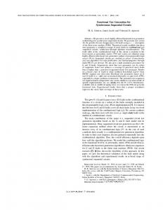
alphabet encodes the environment actions. The distinction between control and disturbance alphabets is essential for providing a flexible framework for robustness analysis of sequential circuits. In particular, it allows to identify parts of the circuit that are wanted to be discontinuous and to eliminate them from the robustness analysis. This is because control actions are expected to cause discontinuities (e.g., in controllers that exhibit switching behavior), and as a consequence, we want to have a framework that only considers the effect of small changes in the disturbance actions. Due to their inherent discontinuous nature, the correctness of control inputs needs to be provided by using other methods that are outside of the scope of this paper, such as the error codes or input replication. The main challenge for defining robustness as a form of continuity is to choose an appropriate notion of distance in the discrete setting. We identify such a metric, that we call common suffix distance. The common suffix distance gives the last position in which two sequences mismatch. Finally, we define what we call ΣD -robustness of sequential circuits as a form of continuity with respect to disturbance actions in the common suffix topology. Intuitively, ΣD -robustness can be viewed as bounded propagation of changes in disturbance inputs: a finite number of changes in the disturbance values results in a bounded number of changes in the computed outputs. We illustrate our notion of ΣD -robustness for sequential circuits with the example of a 2-bit half-adder, which is depicted in Figure I (a). A 2-bit half-adder implements a simple arithmetic function that takes as inputs two boolean data values d1 and d2 and computes their sum and carry values. We model d1 and d2 as disturbance variables. This circuit is clearly ΣD -robust with respect to d1 and d2 because at any time t, the outputs sum and carry depend only on values of d1 and d2 at t. It follows that the effect of a change in input data (d1 and d2 ) at some point in time, is only limited to the computation of output values at that time without being propagated further in the future. In Figure I (b), the half-adder is connected to a small controller that operates as follows: (1) as long as ctr remains low, the half-adder is inactive and sum and carry remain low, (2) when ctr is set to high for the first time, the half-adder is irreversibly activated and from then on, the controlled circuit copies the output values of the half-adder. Switching ctr to high has the qualitative effect on the behavior of the circuit. For instance, a sequence 0ω of ctr values causes the half-adder to remains inactive forever. As a consequence, the output values of sum and carry do not depend on d1 and d2 and always remain low by default. For a sequence 1 · 0ω , that differs from 0ω only in the value of ctr at the first position, the output behavior of the circuit changes drastically. Now, the values of sum and carry represent the result of the half-adder computation on inputs d1 and d2 . In this example, the controller clearly causes discontinuities

in the circuit behavior. However, ctr is a control variable and as such does not affect the ΣD -robustness analysis, and the circuit does remain ΣD -robust with respect to d1 and d2 . This example is a simplified version of a more detailed example described in Section VI. d1 d1 d2

(a)

Figure 1.

sum

d2

carry

ctr

sum

Half Adder

carry

(b)

(a) 2-bit half-adder (b) Controlled 2-bit half-adder

Our definition of ΣD -robustness relates pairs of input sequences that a sequential circuit consumes to the pairs of output sequences that it generates, without explicit reference to the underlying structure of the circuit. We give an alternative structure-less characterization of ΣD -robust sequential circuits that is expressed in terms of the internal memory requirements for the storage of previous inputs in order to be able to compute the output. Given a sequential circuit with a partition of control ΣC and disturbance ΣD input alphabets, we define the class of circuits that have finite disturbance horizon. A circuit has finite disturbance horizon if it has a bound b such that the output at any time is computed as a function of, possibly, all previous control inputs, but only up to b previous disturbance inputs. We show that ΣD -robust sequential circuits coincide exactly with circuits that have finite disturbance horizon. Another contribution of the paper is the characterization of the class of ΣD -robust sequential circuits in the form of their structural properties. This result is obtained by studying ΣD robustness for Mealy machines – a model that corresponds to the class of deterministic and synchronous finite-state transducers. We define a class of ΣD -synchronized Mealy machines and show that is equivalent to corresponding ΣD robust sequential circuits. ΣD -synchronization is an explicit state-based property of Mealy machines. Intuitively, a Mealy machine is ΣD -synchronized if after reading two finite words of the same length with the same control, but possibly differing disturbance components, the machine is guaranteed to reach a “reset” state after reading any sufficiently long (continuation) sequence. The above characterization of ΣD -robust Mealy machines is operational and results in an effective algorithm for checking the ΣD -robustness of arbitrary Mealy machines. The time complexity of the algorithm is quadratic in the number of states of the Mealy machine and the size of its

disturbance alphabet and linear in the size of its control alphabet. Our results have potential for a variety of future work. In this paper, we provide a detailed discussion for two of these directions: studying robustness of asynchronous systems and compositional design. Related work: Robustness of systems has been studied and formalized in many different ways. For example, in [CB02], [KC04] robustness of hybrid systems (mixing discrete and continuous behaviors) is studied as a form of continuity in topologies induced by (extensions of) the Skorokhod distance. The immunity of finite state automata to noise from the external environment has been studied in [DM94], but this study is done in a probabilistic setting. Robustness of finite-state systems has been studied much less in the area of computer science. The work in [BGHJ09] focuses on the synthesis of robust discrete controllers satisfying an extended temporal logic specification with quantitative (real-valued) constraints, which results in a different model of robustness. In the context of real-time systems, robustness has been studied in [GHJ97]. This work differs from ours in that (1) the authors study acceptors (automata) instead of transducers and (2) pairs of timed sequences are compared using the Hausdorff distance with the limitation that the perturbations are allowed only in the time delays between events, while the discrete part has to match exactly. Robustness is also closely related to other research areas such as fault tolerance and error resiliation [SLM09]. In [Mal93], the authors consider combinatorial circuits with cycles, and study conditions under which such circuits can be expressed as an equivalent acyclic circuit. This work can be related to robustness questions since the presence of feedback loops in a circuit is a necessary condition for generating non-robust behavior. Finally, we observe that the problem of robustness can be seen as a dual of the problem of coverage, where one expects that an input change does result in drastic output change [KLS08]. II. P RELIMINARIES We first recall the classical definitions of distance and metric. A distance on a set S is a function d : S × S → R ∪ {∞}. In general, one considers metrics that extend the definition of distance with some natural properties. The distance d is a metric if for all x, y, z ∈ S (1) d(x, y) ≥ 0, (2) d(x, y) = 0 if and only if x = y, (3) d(x, y) = d(y, x), and (4) d(x, y) ≤ d(x, z) + d(z, y). Let Σ = ΣC × ΣD and Γ be (2- and 1-dimensional) finite alphabets. A finite sequence σ ˆ = (c0 , d0 ) · · · (cn−1 , dn−1 ) is an element in Σ∗ where |ˆ σ | = n denotes the length of the sequence. An infinite sequence σ = (c0 , d0 ) · (c1 , d1 ) · · · is an element of Σω . We denote by σ i = (ci , di ) the (i + 1)th letter in a (finite or infinite) sequence σ. Given an infinite sequence σ ∈ Σω , we denote by σ [0,m) the prefix of σ of length m, and by σ m... = σ m σ m+1 . . . its infinite suffix

a p

b w

p

w

w

c d

y

(a)

(b)

z

(c)

Figure 2. Circuits: (a) combinatorial (b) acyclic with delay (c) sequential

from position m on. We denote by πi (σ) = i0 · i1 · · · the projection of sequence σ to its ith component, where i ∈ {c, d}. We similarly define 1-dimensional sequences γ ∈ Γω and γˆ ∈ Γ∗ . Given the alphabets Σ and Γ, a transducer is a function F : Σω → Γω that maps infinite sequences over the alphabet Σ into infinite sequences over Γ. In this paper, we restrict ourselves to sequential finitestate transducers. Such transducers can be seen as finite-state automata [Mea55] whose transitions are labeled by an input and an output letter (see Section IV). III. S EQUENTIAL C IRCUITS AND THEIR ROBUSTNESS In this section, we use sequential circuits [BW53] as an instance of deterministic finite-state transducers with finite alphabet. First, we define their formal model and emphasize some properties of this class of circuits (Section III-A). Then, we consider standard distance functions for string comparison and we show that they do not induce a satisfactory notion of robustness (Section III-B). We introduce the common suffix distance as a new metric (Section III-C) leading to a definition of robustness for sequential circuits with respect to a (disturbance) subset of its input variables, and we give necessary and sufficient conditions for a sequential circuit to be robust (Section III-D). A. Sequential Circuits A combinatorial circuit is a logic circuit that computes a Boolean function of its inputs. It consists of a set of gates and inputs interconnected by a set of wires without cycle. The gates are basic elements that compute simple Boolean functions such as NOT, AND or OR gates. Combinatorial circuits are memoryless by definition, meaning that the value of the output at any (discrete) time instant is a function of the values of its inputs at the same time instant. An example of combinatorial circuit with three NAND gates is shown in Figure 2(a). A sequential circuit is an extension of combinatorial circuits with additional memory devices, called delays. The delay element “shifts” the input values by one time step, thus the output value of a memory device at time t > 0 is equal to its input value at time t − 1. If the circuit contains no cycle (as in Figure 2(b)), we call it an acyclic circuit with delay. In general, sequential circuits can contain cycles, as long as each cycle has at least one delay element.

Control inputs u1 uk ... x1 Disturbance . . . inputs xm

Combinatorial Circuit y1

yn

Figure 3.

delay ... delay

w

z1

zn

A generic sequential circuit C.

Cycles in sequential circuits are called feedback loops (as in Figure 2(c)). Feedback loops in sequential circuits are used to compute the value of the output at time t > 0 as a function of the current value of the inputs, but also of the value of its output at the previous time step t − 1 which is fed back to the circuit through the cycle. Given that the output of the memory devices at any time t > 0 may depend itself on the inputs at time instants t′ < t, the output of a sequential circuit can be a function of both its current and past inputs. Therefore, sequential circuits are best viewed as mappings of input sequences into output sequences. Note that the output of a memory device may not depend at all on any inputs, but be a function of only its own outputs in the previous time step. The set of output values of the delay elements represent the current state of the circuit. A sequential circuit with k memory devices has at most 2k states, or alternatively, a circuit with m states needs at least ⌈log m⌉ delay elements. We now formally define a sequential circuit as a system of equations that describe the relation between inputs, outputs and memory elements, using a standard notation [LMK98], [Brz62]. Our definition of sequential circuits differs from the standard one, in that we make a distinction between control and disturbance input variables. Figure 3 shows a generic sequential circuit. Definition 1: A sequential circuit C with k + m control and disturbance inputs and n delay elements consists of sets U = {u1 , . . . , uk } and X = {x1 , . . . , xm } of control and disturbance variables, a set Y = {y1 , . . . , yn } of current-state variables, a set Z = {z1 , . . . , zn } of next-state variables, an output variable w, and a relation between input, output, and state variables expressed by a set of equations of the form  z1   

zn    w

= ... = =

f1 (u1 , . . . , uk , x1 , . . . , xm , y1 , . . . , yn ) fn (u1 , . . . , uk , x1 , . . . , xm , y1 , . . . , yn ) fC (u1 , . . . , uk , x1 , . . . , xm , y1 , . . . , yn )

where fi and fC are Boolean functions, for i = 1 . . . n. The set {f1 , . . . , fn } is called the transition equations of C and

fC the output equation of C. The next-state variables are updated according to the following equations, where yit and zit denote the valuation of variables yi and zi at time step t:  0 if t = 0 yit = for i = 1 . . . n zit−1 if t > 0 The next lemma states that a sequential circuit can be “unfolded” at any time instant to express the output value as a function of its past and current (control and data) inputs, without explicit reference to the state variables. Lemma 1: Given a sequential circuit C with k+m control and disturbance input variables and n delay elements, and a time instant t ∈ N, the value of the output and state variables in C at time t is a function of its past and current control and disturbance values, that is, there exist functions f t , git : {0, 1}(k+m)×(t+1) → {0, 1} for i = 1 . . . n such that wt = f t (u01 , . . . , u0k , x01 , . . . , x0m , . . . , ut1 , . . . , utk , xt1 , . . . , xtm ) and zit = git (u01 , . . . , u0k , x01 , . . . , x0m , . . . , ut1 , . . . , utk , xt1 , . . . , xtm ) Sequential circuits can also be encoded as functions that map input sequences to output sequences (i.e., transducers). Consider a sequential circuit C with k + m control and disturbance input variables and n memory elements. Let ΣC = {0, 1}k and ΣD = {0, 1}m be the corresponding control and disturbance alphabets. We denote by Σ = ΣC ×ΣD the joint input alphabet where each letter (c, d) ∈ Σ denotes a vector of assignments to the input variables, and by Γ = {0, 1} the output alphabet. The sequential behavior of the circuit C is the function FC : Σω → Γω and we denote by γ = FC (σ) the fact that the output sequence γ ∈ Γω is generated by C on input σ ∈ Σω . By Lemma 1, for all t ≥ 0, we can express γ t as a function of the previously consumed input letters σ [0,t+1) . In the rest of the paper, we use this sequence-oriented definition of the semantics of sequential circuits. B. Hamming and Levenshtein Distances Hamming and Levenshtein distances are standard metrics that have been proposed to measure the similarities between pairs of sequences. In this section, we formally define them and show that they are not appropriate for studying robustness of sequential circuits. Definition 2: Let Σ be a finite alphabet and a1 , a2 ∈ Σ. The Hamming distance between two finite words σ ˆ1 , σ ˆ2 ∈ Σ∗ such that |ˆ σ1 | = |ˆ σ2 |, is defined inductively by dH (ǫ, ǫ) dH (a1 · σ ˆ1 , a2 · σ ˆ2 )

=  0 =

dH (ˆ σ1 , σ ˆ2 ) 1 + dH (ˆ σ1 , σ ˆ2 )

if a1 = a2 if a1 6= a2

The Hamming distance between two infinite words σ1 , σ2 ∈ Σω is [0,n) [0,n) dω , σ2 ). H (σ1 , σ2 ) = lim dH (σ1 n→∞

ΣC = ∅ ΣD = {p, p}

this circuit should not be considered as “robust” because the mismatch occurring in the first position of the pair of input sequences becomes observable only in the (2n + 2)th w position in the pair of output sequences. Since n can be arbitrarily large, it follows that C can propagate “errors” resulting from a noisy input arbitrarily far in the output. p When considering critical systems, we believe that the effect of an input error should be detected and become observable as soon as possible in the output so that the system can be (self) recovered in some predictable amount of time. Figure 4. A sequential circuit C that delays the mismatching input letter Therefore, unbounded delays in error propagation is not in σ1 : p · p2n · p · pω and σ2 : p · p2n · p · pω arbitrarily far in the output. acceptable in most applications and should not be considered as a robust behavior. The reason why neither of the Hamming and Levenshtein Definition 3: Let Σ be a finite alphabet and a1 , a2 ∈ Σ. distances defines a satisfactory metric for robustness of The Levenshtein distance between two finite words σ ˆ1 , σ ˆ2 ∈ sequential circuits is due to the fact that they just count Σ∗ is defined inductively by the absolute number of positions in which two sequences dL (ǫ, σ ˆ2 ) = |ˆ σ2 | mismatch. The information that is not captured by these dL (ˆ σ1 , ǫ) = |ˆ σ | 1 distances is the relative position of the mismatches in the  d (ˆ σ , σ ˆ ) if a = a  L 1 2 1 2 input and output sequences.   min{dL (ˆ σ1 , σ ˆ2 ), if a1 6= a2 dL (a1 · σ ˆ1 , a2 · σ ˆ2 ) = C. Common suffix distance dL (a1 · σ ˆ1 , σ ˆ2 ),    dL (ˆ σ1 , a2 · σ ˆ2 )} + 1 We propose an alternative metric that we call the common suffix distance and that is the last position in which two The Levenshtein distance between two infinite words sequences differ. We note that the common suffix distance ω σ1 , σ2 ∈ Σ is coincides with the inverse of the Cantor distance. [0,m) [0,n) dω , σ2 ) | σ1m... = σ2n... } Definition 4: Let Σ be a finite alphabet. The common L (σ1 , σ2 ) = inf{dL (σ1 suffix distance between two finite words σ ˆ1 , σ ˆ2 ∈ Σ∗ such where inf{∅} = ∞. that |ˆ σ1 | = |ˆ σ2 | is defined inductively by We argue that neither of the two standard distances ds (ǫ, ǫ) =  0 can be used to define a satisfactory notion of robustness ds (ˆ σ1 , σ ˆ2 ) if a1 = a2 for sequential circuits. We illustrate this point with the ds (ˆ σ1 · a1 , σ ˆ2 · a2 ) = |ˆ σ1 | + 1 if a1 6= a2 sequential circuit C shown in Figure 4. This circuit has a single disturbance variable p and an output variable w and The common suffix distance between two infinite sequences behaves as follows: (1) C outputs 1 whenever p is true; σ1 , σ2 ∈ Σω is (2) the first time that the input p becomes false, C outputs [0,n) [0,n) dω lim ds (σ1 , σ2 ). either 0 or 1, depending on whether the current value of the s (σ1 , σ2 ) = n→∞ input sequence p was preceded by an even or odd number The common suffix distance is an upper bound on the of consecutive 1s (3) the output will be 1 no matter the Hamming distance, as for all sequences σ1 , σ2 ∈ Σω , subsequent inputs. Consider the following patterns of input dH (σ1 , σ2 ) ≤ ds (σ1 , σ2 ). Although the common suffix sequences σ1 and σ2 and the corresponding output sequences distance does not count the number of relative differences γ1 = fC (σ1 ) and γ2 = fC (σ2 ) generated by C, where n ≥ 0 between σ 1 and σ2 within their prefix where the mismatchis some arbitrary integer ing occur, it does provide enough information for checking the robustness of a sequential circuit with respect to a subset γ1 : w · w2n · w · wω σ1 : p · p2n · p · pω of its input variables. σ2 : p · p2n · p · pω γ2 : w · w2n · w · wω The following lemma states that the distance between two sequences σ1 , σ2 ∈ Σω is finite (and bounded by some As we can see, in the above example dH (σ1 , σ2 ) = integer k) if and only if σ1 and σ2 have common suffixes dL (σ1 , σ2 ) = 1 and dH (γ1 , γ2 ) = dL (γ1 , γ2 ) = 1, for any from a position strictly smaller than k. value of n. It follows that for this particular pattern of inputs, Lemma 2: For all σ1 , σ2 ∈ Σω and k > 0, dω a mismatching in a pair of input sequences does not cause s (σ1 , σ2 ) < k iff there exists 0 ≤ m < k such that σ1m... = σ2m... . C to increase the number of mismatches in the generated We can show that the common suffix distance defines a outputs. This observation suggests that the circuit is “robust” metric. with respect to Hamming and Levenshtein distances, at Lemma 3: The common suffix distance is a metric. least for this particular pair of input sequences. However,

D. ΣD -Robustness as Finite Disturbance Horizon

ΣD = {p, p}

In this section, we define robustness for sequential circuits as a form of continuity with respect to the disturbance subset of its input variables in the common suffix topology. Our definition relates the positions of mismatching characters in the pairs of input and output sequences, where the two input sequences have the identical control, but possibly different disturbance components. In particular, we ask that there exists a bound b on the propagations of mismatches, namely, that if the last mismatching in the input sequence occurs at position k, then the last mismatching in the output sequence occurs before position k + b. The addition is used in order to make the definition of robustness invariant to the actual positions in which mismatches happen. Definition 5: A sequential circuit C with ΣC and ΣD control and disturbance input alphabets is ΣD -robust if there exists b ≥ 0 such that for all k > 0 and all σ1 , σ2 ∈ (ΣC × ΣD )ω such that πC (σ1 ) = πC (σ2 ), if ω dω s (σ1 , σ2 ) < k, then ds (FC (σ1 ), FC (σ2 )) < k + b. We introduce the class of sequential circuits with finite disturbance horizon. A circuit with control alphabet ΣC and disturbance alphabet ΣD has the finite disturbance horizon property if it has a fixed bound on the number of current and past disturbance inputs that are necessary to determine its output at any time instant. Definition 6: Let FC : (ΣC × ΣD )ω → Γω be the sequential function of a circuit C, where γ = FC (σ). We say that C has finite disturbance horizon if for some bound b, for all time instants t greater than or equal to b, it is sufficient to consider, together with all past control input symbols, the current and previous b disturbance input symbols in order to compute the value of γ t , i.e., there exists b ∈ N such that for all t ≥ b and σ ∈ (ΣC × ΣD )ω , there exists a function Gt : Σt+1 × Σb+1 → Γ, such that C D [0,t+1) [t−b,t+1) t t γ = G (σC , σD ), where σC = πC (σ) and σD = πD (σ). Note that the above definition considers time instants greater than or equal to b. For t < b, the number of previous (control and disturbance) inputs needed to compute the output is trivially bounded by b. Example 1: Consider the circuit in Figure 2(b). It contains no feedback loop and the output function can be expressed as w0 = 0 and wt = 1−pt−1 for all t > 0. It follows that the circuit has finite disturbance horizon, independently on whether p is a control or a disturbance input variable . Indeed, its output function depends only on the value of the input in the previous step. It is easy to see that all acyclic circuits with delay have finite disturbance horizon for any control/disturbance partition of input variables. Example 2: The circuitWshown in Figure 2 (c) contains a t feedback loop and ut = i=0 pi for all t ≥ 0, that is the output at time t depends on the value of all the previous values of p. This circuit is robust only if p is a control and

p

C2

C4

C1 w

C3

Figure 5.

An example of a robust sequential circuit

not a disturbance variable. Example 3: The circuit in Figure 5 has a disturbance variable p and a feedback loop and can be logically decomposed into four components. The circuit C1 implements a modulo 2 counter using a feedback loop and has no input. The circuits C2 and C3 define two sequential functions that are dependent only on the input value in the present and previous time step, respectively. Finally, C4 propagates the output of either C2 or C3 depending on the current value of the counter C1 . The output can be expressed as wt = pt if t is even, and wt = pt−1 if t is odd. Therefore, the whole system implements a sample-and-hold function that propagates the input value at every even time step, and holds it for two instants of time. Although the output at time t depends on the current state of the circuit, it can be computed as a function of some bounded portion of the past inputs. Therefore the circuit has finite disturbance memory. We show in Theorem 1 that a sequential circuit is ΣD robust if and only if it has finite disturbance horizon, that is if it always forgets about disturbance inputs older than some bounded amount of time. The intuition is that an “altered” disturbance input is forgotten by the circuit after some finite time and consequently does not influence the computation of the circuit’s output after that time. Theorem 1: A sequential circuit is ΣD -robust if and only if it has finite disturbance horizon. The next result follows from the fact that combinatorial circuits are memoryless and that acyclic circuits with delay have finite disturbance horizon by definition. Corollary 1: Every combinatorial circuit and every acyclic circuit with delay is ΣD -robust. IV. O PERATIONAL C HARACTERIZATION OF ΣD -ROBUSTNESS FOR S EQUENTIAL C IRCUITS Sequential circuits have an equivalent graphical representation called Mealy machines [Mea55]. Such machines consist of a finite number of states (the internal memory of the circuit) and transitions between the states labeled by

b = |ˆ σs | =

k = |ˆ σ1 | = |ˆ σ2 | πC (ˆ σ1 ) = πC (ˆ σ2 )

|Q|2 −|Q| 2

ΣD = {p, p} p/0

q1 σ ˆ1 /ˆ γ1

A

σ ˆs /ˆ γs1

q0

q

σ ˆ2 /ˆ γ2

p/1

σ/γ

B

p/0

p/0 p/1

D

σ ˆs /ˆ γs2 q2

p/1

C p/1

Figure 7. Figure 6.

p/0

ΣD -synchronization of Mealy machines: Example

ΣD -synchronization of Mealy machines: General case

input/output actions. Mealy machines can be used to model the high-level behavior of the underlying circuit. We propose an alternative characterization of robustness based on the state-based properties of Mealy machines. Formally, Mealy machines are deterministic input/output automata consisting of a finite number of states and a transition relation. Each transition consumes an input symbol and produces an output symbol. Definition 7: A Mealy machine is a tuple M = (Q, ΣC , ΣD , Γ, q0 , δ, λ) where Q is a finite set of states, ΣC and ΣD are control and disturbance input alphabets, Γ is the output alphabet, q0 ∈ Q is the initial state, δ : Q × (ΣC × ΣD ) → Q is the state transition function and λ : Q × (ΣC × ΣD ) → Γ is the output function. The state transition function δ and the output function λ are extended to sequences as follows (inductively): δ(q, (c, d) · σ ˆ ) = δ(δ(q, (c, d)), σ ˆ ) and λ(q, σ ˆ · (c, d)) = λ(δ(q, σ ˆ ), (c, d)) for all (c, d) ∈ (ΣC × ΣD ) and σ ˆ ∈ (ΣC × ΣD )+ . A Mealy machine M defines a function fM : (ΣC × ΣD )ω → Γω in the expected way. The machine M and a sequential circuit C are equivalent if fM (σ) = FC (σ) for all σ ∈ (ΣC × ΣD )ω . M is minimal if for all states q, q ′ ∈ Q such that q 6= q ′ , there exists an input sequence σa ∈ (ΣC × ΣD )+ such that λ(q, σa ) 6= λ(q ′ , σa ). Mealy machines can be minimized in time O(n · log n) where n = |Q| is the number of states [Hop71]. In the sequel, we define a class of Mealy machines (as in Figure 6) that we call ΣD -synchronized. Intuitively, a Mealy machines is ΣD -synchronized if from every pair of states reachable by two input sequences of the same length and with the same control component, a “reset” state is reached after reading any sufficiently long word. Consider the machine M in Figure 7 with ΣD = {p, p}, implementing a delay of length 2. From the initial state A, every state is reachable with some input of length 3. In this particular example, in order to show that the machine is ΣD -synchronized, we need to check that from every pair of its states, a single state is reached with every sufficiently long word. This holds since from every state, the disturbance

input p · p leads to A, p · p to B, p · p to C, and p · p to D. Definition 8: A Mealy machine M is ΣD -synchronized if there exists a bound β ∈ N such that for all σ ˆ1 , σ ˆ2 , σ ˆs ∈ (ΣC ×ΣD )∗ with |ˆ σ1 | = |ˆ σ2 |, πC (ˆ σ1 ) = πC (ˆ σ2 ) and |ˆ σs | ≥ β, we have δ(q0 , σ ˆ1 · σ ˆs ) = δ(q0 , σ ˆ2 · σ ˆs ). It turns out that the class of ΣD -synchronized Mealy machines corresponds exactly to the one of sequential circuits that are ΣD -robust. Theorem 2: A sequential circuit is ΣD -robust if and only if its equivalent Mealy machine is ΣD -synchronized. Moreover, the robustness bound b in Definition 5 and the bound β in Definition 8 coincide. Finally, we show in the proof of Theorem 2 in Appendix A that if the Mealy machine of a sequential circuit is ΣD -synchronized, then 2 we can take β = |Q| 2−|Q| giving the same value for the robustness bound b of the circuit. V. C HECKING ΣD -ROBUSTNESS OF M EALY M ACHINES In this section, we propose a two-step algorithm for checking the ΣD -robustness of minimal Mealy machines. The algorithm is based on a standard graph analysis. Given an arbitrary minimal Mealy machine M = (Q, Σc , Σd , Γ, q0 , δ, λ), the first part of the algorithm is a graph exploration procedure that computes QM , the set that contains all distinct pairs of states in M that are reachable from the initial state q0 by reading two input words of the same length with the same control, but possibly differing disturbance components. QM

= {{q1 , q2 } | q1 , q2 ∈ Q s.t. q1 6= q2 and ∃σa , σb ∈ (ΣC × ΣD )∗ s.t.|σa | = |σb |, πC (σa ) = πC (σb ) and q1 = δ(q0 , σa ) and q2 = δ(q0 , σb )}

We have to check whether there exists a length β such that on all input words σs ∈ (ΣC × ΣD )∗ of length β, from every pair of states {q1 , q2 } in QM , a single state is reached, i.e., δ(q1 , σs ) = δ(q2 , σs ). This is the case 2 only if there exists no word σs of length |Q| 2−|Q| that induces a loop through pairs in QM (otherwise an arbitrarily long word can be constructed that violates the condition of ΣD -synchronization), i.e., that ∀{q1 , q2 } ∈ QM · ∄ σs :

q1 = δ(q1 , σs ) and q2 = δ(q2 , σs ). It follows that the ΣD -robustness of a Mealy machine M can be decided by a cycle detection algorithm on the graph GM (QM , δM ) where δM ⊆ QM × QM and ({q1 , q2 }, {q1′ , q2′ }) ∈ δM iff q1′ = δ(q1 , (c, d)) and q2′ = δ(q2 , (c, d)) and q1′ 6= q2′ for some (c, d) ∈ ΣC × ΣD . The cycle detection can be done on-the-fly with the generation of GM . Theorem 3: The complexity of checking robustness of a minimal Mealy machine M = (Q, ΣC , ΣD , Γ, q0 , δ, λ) is 2 O( |Q| 2+|Q| · |ΣC | · |ΣD |2 ). VI. D ETAILED E XAMPLE An adder-subtractor is a sequential circuit that combines addition or subtraction operations of binary numbers in a single unit. Adders and subtractors are usually part of the arithmetic logic unit (ALU). There is an additional control unit that decides which operation the ALU should perform. a3

b3

a2

b2

a1

b1

a0

b0

subtraction in the first step, and than switches to the addition operation in the next step and remains doing addition forever. On the other hand, the second input sequence makes the circuit doing subtraction forever. As a consequence, the common suffix distance between the two input sequences is 1, but the output sequences drastically differ, given that they are computed using a different operation. This circuit can be made ΣD -robust with respect to all inputs by changing the encoding of the control signal d. Instead of having the environment that provides the information when to switch from addition to subtraction and vice versa, we can design a circuit that expects from the environment explicit request about which operation to apply at each step. In this case, we do not need the switch control unit and the control input can be directly fed to the ALU. Any error in the control signal would then affect only the computation of the output at the time step of the error occurrence, but would not propagate to the future computation of the output. VII. D ISCUSSION

switch 1

c4

0

1

1−bit Full Adder

s3

c3

0

1

1−bit Full Adder

s2

Figure 8.

c2

0

1

1−bit Full Adder

s1

c1

0

d

1−bit Full Adder

c0

s0

A 4-bit ripple carry adder-subtractor

The 4-bit adder-subtractor shown in Figure VI, the circuit is composed of four 1-bit full adders and a control unit switch. It combines the adding and subtracting capabilities by exploiting the fact that when the numbers are in two’s complement, it is sufficient to invert each bit with a NOT gate and add 1, to implement subtraction using the adders. The circuit takes as inputs variables a0 , . . . , a3 and b0 , . . . , b3 and outputs their sum or difference in the output variables s0 , . . . , s3 , together with a carry output c4 . The function that is computed by the circuit depends on the switch control unit that takes as input the signal d. Initially, the circuit is set to do addition. Whenever d is set to high, the circuit switches to the other function. Intuitively, the input variables in this circuit are naturally partitioned into sets U = {d} and X = {a0 , b0 , . . . , a3 , b3 } of control and disturbance variables, respectively. The circuit is clearly ΣD -robust under this partition, because 1-bit full adders are combinatorial circuits without memory. However, if we assume that the external environment is not fully reliable, and may introduce errors in the d signal, we cannot consider d anymore a control, but rather a disturbance variable. In that case, the circuit is not ΣD -robust anymore. For this, consider two input sequences of d, σd : 110ω and σd′ : 10ω . In the first case, the circuit switches to do the

This section briefly discusses two extensions of the results presented for sequential circuits. We first add insertion and deletion operators to the common suffix distance and study how it affects the ΣD -robustness of sequential circuits. We observe that this distance is not adapted to synchronous systems. Second, we discuss about the preserving of ΣD robustness properties of individual sequential circuits by their composition. A. Effect of the Edit Operations to the ΣD -Robustness of Sequential Circuits In Section III-C, we introduced the common suffix distance that considers only the last substitution of characters in a pair of sequences. In this section, we define the edit common suffix distance that extends the common suffix distance with additional edit operations (insertion and deletion). This extension is analogous to the Levenshtein extension of the Hamming distance. Edit operations are natural to model the effect of the environment providing to the system sequences with missing or redundant inputs. Definition 9: Let Σ be a finite alphabet. The edit common suffix distance between two finite words σ ˆ1 , σ ˆ2 ∈ Σ∗ is defined inductively by = |ˆ σ2 | =  |ˆ σ1 | des (ˆ σ1 , σ ˆ2 ) des (a1 · σ ˆ1 , a2 · σ ˆ2 ) = max{|ˆ σ1 |, |ˆ σ2 |} + 1 des (ǫ, σ ˆ2 ) des (ˆ σ1 , ǫ)

if a1 = a2 if a1 6= a2

The edit common suffix distance between two infinite words σ1 , σ2 ∈ Σω is [0,m)

dω es (σ1 , σ2 ) = inf{des (σ1

[0,n)

, σ2

) | σ1m... = σ2n... }.

We note that the edit common suffix distance is an upper bound on the Levenshtein distance, as for all sequences σ1 , σ2 ∈ Σω , dL (σ1 , σ2 ) ≤ des (σ1 , σ2 ). We first show that sequential circuits that do not have feedback loops are not sensitive to insertion and deletion operations and remain ΣD -robust with respect to the edit common suffix distance. Theorem 4: Acyclic circuits with delay are ΣD -robust with respect to the edit common suffix distance. However, sequential circuits with feedback that are ΣD robust with respect to common suffix distance may be very sensitive to edit operations. We illustrate this point with the circuit C from Figure 5 that is ΣD -robust with respect to the common suffix distance. We assume that ΣD = {p, p}. Consider the following input and output sequences γ1 = fC (σ1 ) and γ2 = fC (σ2 ), where σ2 = p · σ1 σ1 : p · p · p · · · σ2 : p · p · p · p · · ·

γ1 : w · w · w · · · γ2 : w · w · w · w · · ·

As we can see, a simple insertion of a single letter at the beginning of the input sequence results in a completely different output sequence, i.e. dω es (σ1 , σ2 ) = 1 but dω (γ , γ ) = ∞. In fact, sequential circuits are synchronous 1 2 es systems with a global clock. While substituting an input with another one does not affect the clock of the circuit, inserting or deleting a letter in the input sequence of a sequential circuit “shifts” the global clock of the system. Synchronous systems that compute their output as a function of their disturbance input and internal clock value (the value of a state-based modulo counter) are in general very sensitive to such clock shifts and result in producing non-ΣD -robust output behavior. We note that the edit common suffix distance may be well-adapted to the study of robustness of asynchronous systems that do not have a global clock. We believe that such asynchronous systems should be less sensitive to the shifts caused by the insertions and deletions of disturbance values in the input sequence. B. Composition of Sequential Circuits In this paper, we studied the ΣD -robustness of sequential circuits as individual components. However, several circuits are generally composed in order to build more complex systems. This observation results in natural questions about the preserving of ΣD -robustness by composition of sequential circuits: (1) What are the conditions for the composition of two ΣD -robust components to remain ΣD -robust? (2) What are the conditions for making a ΣD -robust composition out of two possibly ΣD -non-robust components? Consider the example shown in Figure 9. Figure 9 (a) depicts an OR and AND gate and a delay element. It is easy to see that these basic gates are robust if all their inputs are disturbance variables. A particular composition of the

C

C

C′

(a)

(b)

(c)

Figure 9. Composition of sequential circuits; (a) basic gates (b) ΣD -nonrobust circuit C and (c) ΣD -robust circuit C ′

OR gate with a delay element results in the circuit C that introduces a feedback loop and is depicted in Figure 9 (b). This circuit corresponds to Circuit C given in Figure 2 (c) and we have seen that C is not ΣD -robust. Finally, C can be composed with an additional AND gate and a delay element to obtain the sequential circuit C ′ , shown in Figure 9 (c), that is equivalent to a simple delay element, and is hence ΣD -robust. From this example, we can observe that; (1) the composition of two ΣD -robust circuits may be ΣD -nonrobust and (2) a ΣD -non-robust circuit that is combined with another circuit may result in a ΣD -robust composition. Thus, in general, the composition of sequential circuits preserves neither the ΣD -robustness nor the ΣD -non-robustness of its components. However, the acyclic composition of two ΣD robust component always results in a robust system, since acyclic composition cannot introduce infinite input memory horizon.

VIII. C ONCLUSION AND F UTURE W ORK We proposed a flexible framework for studying the robustness of sequential circuits. Acknowledging the fact that some variables in the circuit are intended to be discontinuous, we partition input variables into two sets of control and disturbance variables, and study robustness only with respect to disturbance inputs. We defined the notion of ΣD robustness for sequential circuits that allows to bound the difference between the distance of pairs of (disturbance) input behaviors and their corresponding output behaviors. Our notion relies on a metric that permits to distinguish substitutions of data in sequences as well as their relative positions, but does not consider suppression and insertion operations. We characterized a non-trivial class of sequential circuits that are ΣD -robust and identified that the ΣD -robustness property is dependent on the horizon of memory that is used within the circuit. An operational characterization of ΣD -robustness based on the analysis of Mealy machines resulted in relating the notion of ΣD -robust input/output finite-state transducers to the well-known problem of synchronizing sequences in deterministic automata. Furthermore, this automata-based approach allowed designing a polynomial-time algorithm for checking the robustness of Mealy machines.

We also study an extension of our distance that allows to take insertion and suppression of information into account. We show that this distance is not natural for sequential circuits which are in general very sensitive to shifts in the synchronous global clock (the position in which events occur). We believe this notion is more adapted to asynchronous circuits, and we left this study for future work. A natural extension of our work would be to study the logical and algebraic characterization of robustness and identify the subset of ω-regular languages that are robust with respect to the distance measures described in this paper. Another important direction for future research is to study quantitative extensions of sequential circuits such as continuous-time sequential circuits [PRT04] or probabilistic circuits,[PM75]. One could obtain a logical characterization of such circuits by using the quantitative and probabilistic languages introduced in [CDH08], [CDH09]. It would be also interesting to be able to distinguish between systems that are robust. As an example, consider two robust circuits C1 and C2 . Assume that the two circuits generate the same behaviors for a given subset I of expected inputs, but may generate different behaviors for inputs that are outside of I. It could be that the b in the distance is the same for both C1 and C2 , but that this b is only reached when reading a few sequences outside of I in C1 and all the sequences outside of I in C2 . In this situation, one should conclude that it is better to use C1 than C2 . Indeed, for input sequences that are outside of I, C1 recovers faster than C2 . The common suffix distance cannot make such distinctions and should be further refined in order to be able to quantify the degree of robustness of such circuits. R EFERENCES [BGHJ09] R. Bloem, K. Greimel, T. A. Henzinger and B. Jobstmann, Synthesizing Robust Systems, In FMCAD’09, 2009. [Brz62] J. A. Brzozowski, Regular Expression Techniques for Sequential Circuits, PhD Dissertation, University of Priceton, 1962. [BW53] A. W. Burks and J. .B. Wright, Theory of logical nets, In IRE’53, 1357–1365, 1953. [CB02] P. Caspi and A. Benveniste, Toward an approximation theory for computerised control, In EMSOFT02, 2491, 2002. [CDH08] K. Chatterjee, L. Doyen and T. A. Henzinger, Quantitative Languages, IN CSL’08, 385–400. [CDH09] K. Chatterjee, L. Doyen and T. A. Henzinger, Probabilistic Weighted Automata, In CONCUR’09, 244–258, 2009. [DM94] B. Delyon and O. Maler, On the Effects of Noise and Speed on Computations, In Theoretical Computer Science, 129, 279-291, 1994 [GHJ97] V. Gupta, T. A. Henzinger and R. Jagadeesan, Robust timed automata. In Hybrid and Real-Time Systems, LNCS 1201, 331–345, 1997.

[Ham50] R. W. Hamming, Error detecting and error correcting codes. In Bell System Technical Journal, 29 (2), 147160, 1950. [Hen08] T. A. Henzinger, Two challenges in embedded systems design: Predictability and robustness, In Philosophical Transactions of the Royal Society, 366, 3727–3736, 2008. [Hop71] J. E. Hopcroft, An n · log n algorithm for minimizing states in a finite automaton, Technical Report CS-71-190, Stanford University, 1971. [KC04] C. Kossentini and P. Caspi, Approximation, sampling and voting in hybrid computing systems, In HSCC’04, 363–376, 2004. [KLS08] O.Kupferman, W.Li and S.A.Seshia, A theory of mutations with applications to vacuity, coverage, and fault tolerance, In FMCAD ’08, 1–9, 2008. [Lev66] V. I. Levenshtein, Binary codes capable of correcting deletions, insertions, and reversals. Soviet Physics Doklady, 10, 707710, 1966. [Lev96] W. S. Levine, The Control Handbook. New York: CRC Press, 1996. [LMK98] G. Langholz, J. L. Mott and A. Kandel, Foundations of Digital Logic Design, World Scientific Publishing, 1998. [Mal93] S. Malik, Analysis of cyclic combinatorial circuits, In ICCAD’93, 618–625, 1993. [Mea55] G. H. Mealy, A method for synthesizing sequential circuits, In Bell Systems Technical Journal, 1045–1079, 1955. [PM75] K. P. Parker and E. J. McCluskey, Analysis of Logic Circuits with Faults Using Input Signal Probabilisties, In IEEE transaction in Computer Science, 573–578, C-24, 1975. [PRT04] D. Pardo, A. M. Rabinovich and B. A. Trakhtenbrot, Synchronous circuits over continuous time: feedback reliability and completeness, In Fundamenta Informaticae, 62(1), 123– 137, 2004. [SLM09] S. A. Seshia, W. Li and S. Mitra, Verification-guided soft error resilience, In DATE ’07, 1442–1447, 2007. ˇ y [Vol08] M. V. Volkov, Synchronizing automata and the Cern` conjecture. In LATA’08, 11–27, 2008.

A PPENDIX Lemma 1: Given a sequential circuit C with k + m control and disturbance input variables and n delay elements, and a time instant t ∈ N, the value of the output and state variables in C at time t is a function of its past and current control and disturbance values, that is, there exist functions f t , git : {0, 1}(k+m)×(t+1) → {0, 1} for i = 1 . . . n such that wt = f t (u01 , . . . , u0k , x01 , . . . , x0m , . . . , ut1 , . . . , utk , xt1 , . . . , xtm ) and zit = g t (u01 , . . . , u0k , x01 , . . . , x0m , . . . , ut1 , . . . , utk , xt1 , . . . , xtm ) Proof: The proof proceeds by induction on the time step t. For the base case, consider t = 0. By the definition of a sequential circuit, yi0 = 0 for i = 1 . . . n. It follows that in w0 = fC (u01 , . . . , u0k , x01 , . . . , x0m , y10 , . . . , yn0 ) , all yi0 can be replaced by the constant 0, and fC can be expressed in terms of an equivalent function f such that w0 = f (u01 , . . . , uk , x01 , . . . , x0m ). The proof is similar for zi0 . For the inductive hypothesis, assume that for an arbitrary t > 0, there exists a function f such that wt = f (u01 , . . . , u0k , x01 , . . . , x0m , . . . , ut1 , . . . , utk , xt1 , . . . , xtm ) and functions gi for i = 1 . . . n such that zit = gi (u01 , . . . , u0k , x01 , . . . , x0m , . . . , ut1 , . . . , utk , xt1 , . . . , xtm ) By definition of a sequential circuit, t+1 t+1 t+1 t+1 t+1 wt+1 = fC (ut+1 1 , . . . , uk , x1 , . . . , xm , . . . , y1 , . . . , yn )

and by inductive hypothesis yit+1 = zit = gi (u01 , . . . , u0k , x01 , . . . , x0m , . . . , ut1 , . . . , utk , xt1 , . . . , xtm ) for i = 1 . . . n. It follows that we can replace every yit+1 in fC by gi (u01 , . . . , u0k , x01 , . . . , x0m , . . . , ut1 , . . . , utk , xt1 , . . . , xtm ) for i = 1 . . . n. Hence fC at t + 1 can be expressed by another function f such that t+1 t+1 t+1 wt+1 = f (u01 , . . . , u0k , x01 , . . . , x0m , . . . , ut+1 1 , . . . , uk , x1 , . . . xm )

. The proof is similar for zit+1 . m... Lemma 2: For any σ1 , σ2 ∈ Σω and k > 0, dω = σ2m... . s (σ1 , σ2 ) < k iff there exists 0 ≤ m < k such that σ1 Proof: Assume that for two arbitrary σ1 , σ2 ∈ Σω , dω (σ , σ ) < k for some k > 0. Assume that there does not exist 1 2 s 0 ≤ m < k such that σ1m... = σ2m... , that is there exists l ≥ k − 1, such that σ1l 6= σ2l . By the definition of the common suffix [0,l+1) [0,l+1) [0,n) [0,n) distance, it follows that ds (σ1 , σ2 ) ≥ k and consequently limn→∞ ds (σ1 , σ2 ) must be greater or equal then k, hence a contradiction with the initial assumption. Therefore, there exists 0 ≤ m < k such that σ1m... = σ2m... . For the other direction of the proof, assume that for arbitrary σ1 , σ2 ∈ Σω , there exist 0 ≤ m < k for some k > 0 such [0,m) [0,m) m... , σ2m... ) = 0. , σ2 ) ≤ m and (2) dω that σ1m... = σ2m... . By the definition of the common suffix distance, (1) ds (σ1 s (σ1 ω ω By combining (1) and (2), it follows that ds (σ1 , σ2 ) ≤ m, that is ds (σ1 , σ2 ) < k and this concludes the proof. Lemma 3: Common suffix distance is a metric. Proof: We only show the fourth requirement of the definition of a metric. For arbitrary σ1 , σ2 , σ3 ∈ Σω , let dω s (σ1 , σ2 ) = c1 ... = σ2c1 ... and σ2c2 ... = σ3c2 ... . Combining c1 and dω s (σ2 , σ3 ) = c2 and c = max(c1 , c2 ). By Lemma 2, it follows that σ1 the two observations, we have that σ1c... = σ3c... and by Lemma 2 that dω s (σ1 , σ3 ) = c = max(c1 , c2 ). It follows that ω ω dω s (σ1 , σ3 ) ≤ ds (σ1 , σ2 ) + ds (σ2 , σ3 ) and this concludes the proof. Theorem 1: A sequential circuit C is ΣD -robust if and only if it has finite disturbance horizon. Proof: Assume that C has finite disturbance horizon. Consider two arbitrary σ1 , σ2 ∈ (ΣC × ΣD )ω such that πC (σ1 ) = πC (σ2 ) and dω s (σ1 , σ2 ) < k for some k > 0, and let γ1 = FC (σ1 ) and γ2 = FC (σ2 ). Then by Lemma 2, there exists m < k such that σ1m... = σ2m... . By the assumption that C has finite disturbance horizon, we know that there exists some b ≥ 0 such that for [n−b,n+1) [0,n+1) [n−b,n+1) [0,n+1) ), where σC1 = πC (σ1 ), σD1 = πD (σ1 ), , σ D2 ) and γ2n = Gn (σC2 , σ D1 all n > m + b, γ1n = Gn (σC1

i i σC2 = πC (σ2 ) and σD2 = πD (σ2 ). By assumption that dω s (σ1 , σ2 ) < k, it follows that σD1 = σD2 for n − b ≤ i ≤ n. i i Furthermore, by the assumption that πC (σ1 ) = πC (σ2 ), it follows that σC = σ for 0 ≤ i ≤ n. Therefore, by definition C2 1 m+b+1... m+b+1... n n . By Lemma 2, we = γ2 of finite disturbance horizon, it follows that γ1 = γ2 for all n > m + b, that is γ1 can conclude that dω s (FC (σ1 ), FC (σ2 )) < k + b and that C is ΣD -robust. For the other direction of the proof, we proceed by contradiction. Assume that C is ΣD -robust and choose a b ≥ 0 such ω that for all k > 0, σ1 , σ2 ∈ Σω with πC (σ1 ) = πC (σ2 ), dω s (σ1 , σ2 ) < k implies ds (FC (σ1 ), FC (σ2 )) < k + b. Assume ω that C does not have finite disturbance horizon, that is for all σ ∈ Σ there exists t ≥ 0 such that γ t cannot be computed [0,t+1) [t−b,t+1) with σC and σD input sequences, where σC = πC (σ) and σD = πD (σ). It follows that γ t must be computed [0,t+1) [t−n,t+1) [0,t+1) [t−n,t+1) n+1 with σC and σD , for some n > b, that is γ t = Gt (σC , σD ) for some Gt : (Σt+1 C × ΣD ) → Γ. ∗ Choose σ ˆ1 , σ ˆ2 ∈ Σ such that πC (ˆ σa ) = πC (ˆ σb ) and ds (ˆ σ1 , σ ˆ2 ) = t − b. Let σ1 = σ ˆ1 · σ, σ2 = σ ˆ2 · σ, γ1 = FC (σ1 ) and γ2 = FC (σ2 ) where σ ∈ Σω is chosen such that γ1t 6= γ2t . Such a σ can be chosen because C is deterministic and we have from ds (ˆ σ1 , σ ˆ2 ) = t − b that σ1t−b−1 6= σ2t−b−1 . But in that case, we have that dω s (σ1 , σ2 ) < t − b + 1 while ω ds (γ1 , γ2 ) ≥ t + 1 which is a contradiction with the assumption that C is ΣD -robust. It follows that if C is ΣD -robust, then C has finite disturbance horizon.

Theorem 2: A sequential circuit C is ΣD -robust if and only if its equivalent Mealy machine M is ΣD -synchronized. Proof: To simplify the presentation, The state transition function δ and the output function λ are extended to sequences as follows (inductively): δ(q, ((c, d) · σ ˆ ) = δ(δ(q, (c, d)), σ ˆ ) and λ(q, σ ˆ · (c, d)) = λ(δ(q, σ ˆ ), (c, d)) for all (c, d) ∈ (ΣC × ΣD ) and σ ˆ ∈ (ΣC × ΣD )+ . Assume that C is ΣD -robust. Consider arbitrary σ ˆ1, σ ˆ 2 ∈ (ΣC × ΣD )∗ such that |ˆ σ1 | = |ˆ σ2 | and πC (ˆ σ1 ) = πC (ˆ σ2 ). We have by definition of the common suffix distance that ds (ˆ σ1 , σ ˆ2 ) < k where k = |ˆ σ1 |+1. By Lemma 2, it follows that for any σ ∈ Σω , dω σ1 · σ, σ ˆ2 · σ) < k. The assumption that C is ΣD -robust and the previous observation s (ˆ σ1 · σ), FC (ˆ σ2 · σ)) < k + b. Consider σ1 · σ, σ ˆ2 · σ) < k and dω imply that there exists b ≥ 0, such that for all σ ∈ Σω , dω s (FC (ˆ s (ˆ ∗ an arbitrary σ ˆs ∈ Σ such that |ˆ σs | ≥ b. Let q1 = δ(q0 , σ ˆ1 · σ ˆs ) and q2 = δ(q0 , σ ˆ2 · σ ˆs ) and assume that q1 6= q2 . Since M is minimal, it follows that there exists σ ˆc ∈ Σ+ such that λ(q1 , σ ˆc ) 6= λ(q2 , σ ˆc ). Combining the previous observations, we ω construct two sequences σ1 , σ2 ∈ Σ such that σ1 = σ ˆ1 · σ ˆs · σ ˆc · σ ′ and σ2 = σ ˆ2 · σ ˆs · σ ˆc · σ ′ where σ ′ ∈ Σω is an arbitrary ω infinite sequence. Let γ1 = λ(q0 , σ1 ) and γ2 = λ(q0 , σ2 ). It follows that ds (σ1 , σ2 ) < k but dω s (γ1 , γ2 ) ≥ k + b because γ1 and γ2 differ at a position greater that |ˆ σ1 | + |ˆ σs |, hence a contradiction with the assumption that q1 6= q2 . It follows that if M is ΣD -robust, there exists b ≥ 0 such that for any σ ˆ1 , σ ˆ2 , σ ˆs ∈ Σ∗ with |ˆ σ1 | = |ˆ σ2 |, πC (ˆ σ1 ) = πC (ˆ σ2 ) and |ˆ σs | ≥ b, δ(q0 , σ ˆ1 · σ ˆs ) = δ(q0 , σ ˆ2 · σ ˆs ). 2 What remains to be shown is that for M with |Q| states, it is sufficient that b = |Q| 2−|Q| . 1) Let q1 = δ(q0 , σ ˆ1 ) and q2 = δ(q0 , σ ˆ2 ) for arbitrary σ ˆ1 , σ ˆ2 ∈ (ΣC × ΣD )∗ such that |ˆ σ1 | = |ˆ σ2 | and πC (ˆ σ1 ) = πC (ˆ σ2 ). |Q|2 −|Q| 2) For M with |Q| states, there are pairs of states (q , q ) such that q = 6 q and (q , q ) = (q , q ). i j i j i j j i 2 2 3) Let σ ˆs ∈ (ΣC × ΣD )∗ be an arbitrary word with |ˆ σs | = |Q| 2−|Q| . We denote σ ˆs = (c0 , d0 ) · · · (c|ˆσs |−1 , d|ˆσs |−1 ) where (ci , di ) ∈ ΣC × ΣD . |ˆ σ | |ˆ σ | 4) Let q1 s = δ(q1 , σ ˆs ) and q2 s = δ(q2 , σ ˆs ) where (c0 ,d0 )

(c1 ,d1 )

(c|ˆ σs |−1 ,d|ˆ σs |−1 )

|ˆ σs |

(c0 ,d0 )

(c1 ,d1 )

(c|ˆ σs |−1 ,d|ˆ σs |−1 )

|ˆ σs |

q1 −−−−→ q11 −−−−→ · · · −−−−−−−−−−−→ q1 and

q2 −−−−→ q21 −−−−→ · · · −−−−−−−−−−−→ q2 |ˆ σ |

|ˆ σ |

5) Assume that q1 s 6= q2 s . Then there exists 0 < m < n ≤ |ˆ σs | such that (q1m , q2m ) = (q1n , q2n ). [0,m) [m,n) i [0,m) [m,n) i m m 6) It follows that q1 = δ(q1 , σ ˆs · (ˆ σs ) ) and q2 = δ(q2 , σ ˆs · (ˆ σs ) ) for any i > 0. [0,m) [m,n) i b 7) Then for any b ≥ 0, one can construct a word σ ˆc = σ ˆs · (ˆ σs ) with i ≥ ⌈ n−m ⌉, that is |ˆ σc | ≥ b such that δ(q0 , σ ˆ1 · σ ˆc ) 6= δ(q0 , σ ˆ2 · σ ˆc ), hence a contradiction with the previous result. It follows that if C is ΣD -robust, then for any σ ˆ1 , σ ˆ2 , σ ˆs ∈ (ΣC × ΣD )∗ with |ˆ σ1 | = |ˆ σ2 |, πC (ˆ σ1 ) = πC (ˆ σ2 ) and |ˆ σs | ≥ |Q|2 −|Q| , δ(q , σ ˆ · σ ˆ ) = δ(q , σ ˆ · σ ˆ ). 0 1 s 0 2 s 2 For the other direction of the proof, assume that M is ΣD -synchronized. Consider two arbitrary sequences σ1 , σ2 ∈ Σω and assume that πC (σ1 ) = πC (σ2 ) and dω s (σ1 , σ2 ) < k for some k > 0. Then by Lemma 2, there exists 0 ≤ m < k such that σ1m... = σ2m... . It follows that we can decompose σ1 and σ2 into sequences σ1 = σ ˆ1 · σ ˆs · σ and σ2 = σ ˆ2 · σ ˆs · σ where

[0,m)

[0,m)

[m,b)

2

σ ˆ 1 = σ1 , σ ˆ 2 = σ2 , σ ˆ s = σ1 , σ = σ1b... and b = m + |Q| 2−|Q| . Let γˆ1 = λ(q0 , σ ˆ1 · σ ˆs ), γˆ2 = λ(q0 , σ ˆ2 · σ ˆs ), γ1 = λ(q0 , σ1 ) and γ2 = λ(q0 , σ2 ). By the definition of the common suffix distance, ds (ˆ γ1 , γˆ2 ) < |ˆ σ1 | + |ˆ σs | + 1, that is 2 ˆ1 · σ ˆs ) = δ(q0 , σ ˆ2 · ds (ˆ γ1 , γˆ2 ) < ds (ˆ σ1 , σ ˆ2 ) + |Q| 2−|Q| . By the assumption that M is ΣD -synchronized, it follows that δ(q0 , σ |Q|2 −|Q| ω ω σ ˆs ). Since M is deterministic, it follows that dω (γ , γ ) = d (ˆ γ , γ ˆ ), concluding that d (γ , γ ) < d (σ , σ ) + . 1 2 s 1 2 1 2 1 2 s s s 2 Theorem 3: The complexity of checking robustness of a minimal Mealy machine M = (Q, ΣC , ΣD , Γ, q0 , δ, λ) is 2 O( |Q| 2+|Q| · |ΣC | · |ΣD |2 ). 2 Proof: Follows from the fact that Algorithm 1 has to consider at most |Q| 2+|Q| states and pairs of states in M multiplied by |ΣC | · |ΣD |2 transitions/pairs of transitions to compute the set QM , which is added to the run time of Algorithm 2 which 2 explores at most |Q| 2−|Q| pairs of states in M and from each explored pair of states has to compute i|ΣC | · |ΣD | transitions. Theorem 4: Acyclic circuits with delay are ΣD -robust with respect to the edit common suffix distance. Proof: Let C be an acyclic circuit with delay. Since C does not have feedback loops, it must define a sequential function that at any time t depends only on its current and previous control and disturbance inputs bounded by b, the number of [t−b,t+1) [t−b,t+1) delay elements. It follows that there exists G : (ΣbC × ΣbD ) → Γ, such that for all t ∈ N, γ t = G(σC , σD ). ω Consider two arbitrary σ1 , σ2 ∈ Σ such that des (σ1 , σ2 ) < k for some k > 0. It follows from Definition 9 that ′ ′ ′ there exist m, n < k such that σ1m... = σ2n... . Then, for every b′ ≥ b, we have γ1b +m = G(σ1b −b+m , . . . , σ1b +m ) and ′ ′ ′ ′ ′ ′ ′ ′ ′ γ2b +n = G(σ2b −b+n , . . . , σ2b +n ). Given that σ1b −b+m = σ2b −b+n , . . . , σ1b +n = σ2b +n , it follows that γ1b +m = γ2b +n , that is γ1m+b... = γ2n+b... and by Definition 9, des (γ1 , γ2 ) < k + b and this concludes the proof. The set QM contains all distinct states and pairs of states in M that are reachable from the initial state q0 by applying to M two input words of the same length with the same control, but possibly different disturbance component. This set is computed with Algorithm 1. The algorithm explores the state-space of M as follows; it starts from the initial state q0 and explores all the neighboring states and pairs of states reachable by the applying letters (c, d1 ), (c, d2 ) ∈ ΣC ×ΣD . From each neighboring state/pair of states the procedure is repeated, until computing all reachable states/pairs of states in M. Every state and pair of states in M is explored at most once. It is not hard to see that the algorithm explores at most |Q| states 2 and |Q| 2−|Q| distinct pairs of states in M, while from any visited state/pair of states one needs to consider |ΣC | · |ΣD |2 outgoing transitions, corresponding to all possible combinations of pairs of (c, d1 ), (c, d2 ) where c ∈ ΣC and d1 , d2 ∈ ΣD . Algorithm 1 Compute QM : C OMP Q M(M) 1: QM ← ∅ 2: V ← {q0 } 3: E ← ǫ, E.enq({q0 }) 4: while (!E.isEmpty()) do 5: {q1 , q2 } = E.deq() 6: for all c ∈ ΣC do 7: for all d1 , d2 ∈ ΣD do 8: q1′ = δ(q1 , (c, d1 )) and q2′ = δ(q2 , (c, d2 )) 9: if {q1′ , q2′ } 6∈ V then 10: E.enq({q1′ , q2′ }) 11: V ← V ∪ {q1′ , q2′ } 12: end if 13: if q1′ 6= q2′ and {q1′ , q2′ } 6∈ QM then 14: QM ← QM ∪ {q1′ , q2′ } 15: end if 16: end for 17: end for 18: end while 19: return QM Algorithm 2 first computes the set QM using the procedure C OMPUTE Q M defined above. Than it generates on-the-fly 2 the graph GM defined in Section V and checks for cycles between pairs of states in QM . It explores at most |Q| 2−|Q| pairs of states and from each state/pair of states has to consider |ΣC | · |ΣD | transitions.

Algorithm 2 Checking the robustness of M : ROBUST(M) 1: V ← ∅ 2: E ← ǫ 3: QM ← C OMPUTE Q M(M) 4: for all {q1 , q2 } ∈ QM do 5: E.enq({q1 , q2 }) 6: V ← V ∪ {q1 , q2 } 7: end for 8: while (!E.isEmpty()) do 9: {q1 , q2 } = E.deq() 10: for all (c, d) ∈ ΣC × ΣD do 11: q1′ = δ(q1 , (c, d)) and q2′ = δ(q2 , (c, d)) 12: if q1′ = q2′ then 13: skip 14: else if {q1′ , q2′ } ∈ V then 15: return NON - ROBUST 16: else if {q1′ , q2′ } 6∈ V and q1′ 6= q2′ then 17: V ← V ∪ {q1′ , q2′ } 18: E.enq({q1′ , q2′ }) 19: end if 20: end for 21: end while 22: return ROBUST