Role of the sample thickness in planar crack propagation

Role of the sample thickness in planar crack propagation Pallab Barai Department of Mechanical Engineering Texas A& M University College Station, TX, USA 77843

Phani K. V. V. Nukala Computer Science and Mathematics Division, Oak Ridge National Laboratory, Oak Ridge, TN 37831-6359, USA

Mikko J. Alava COMP Center of Excellence, Department of Applied Physics, Aalto University, P.O. Box 14100, FIN-00076, Aalto, Espoo, Finland

arXiv:1307.1227v1 [cond-mat.dis-nn] 4 Jul 2013

Stefano Zapperi CNR - Consiglio Nazionale delle Ricerche, IENI, Via R. Cozzi 53, 20125, Milano, Italy and ISI Foundation, Via Alassio 11/c 10126 Torino, Italy We study the effect of the sample thickness in planar crack front propagation in a disordered elastic medium using the random fuse model. We employ different loading conditions and we test their stability with respect to crack growth. We show that the thickness induces characteristic lengths in the stress enhancement factor in front of the crack and in the stress transfer function parallel to the crack. This is reflected by a thickness-dependent crossover scale in the crack front morphology that goes from from multi-scaling to self-affine with exponents in agreement with line depinning models and experiments. Finally, we compute the distribution of crack avalanches which is shown to depend on the thickness and the loading mode. I.

INTRODUCTION

Understanding the failure of disordered media still represent an open problem for basic science and engineering. From the point of view of statistical mechanics, the problems represents an interesting example of the interplay between disorder and long-range interactions and has thus attracted a wide interest in the past years [1]. Fracture typically displays intriguing size-effects and it is not easy to formulate a general law that can predict the the dependence of the failure strength on the relevant lengthscales of the problem, such as the size of the notch, of the fracture process zone and of the sample width and thickness [2–4] Scale and size dependence also permeate the analysis of crack morphologies, that have been originally characterized by self-affine scaling [5, 6], but a complete understanding of the universality classes of the roughens exponent is still an debated issue (for a review see [7]). The prevalent interpretation of experimental measurements for out-of-plane three dimensional cracks suggests a roughness exponent value ζ ≃ 0.8 for rupture processes occurring inside the fracture process zone (FPZ), where elastic interactions would be screened, crossing over at large scales to ζ ≃ 0.4 when elastic interaction would dominate [8, 9]. Furthermore, the fracture surface has been shown to be anisotropic with different scaling exponents in the directions parallel or perpendicular to the crack [8]. A particularly interesting and conceptually simpler example of crack roughening is represented by the propagation of a planar crack. This case appears to be the ideal candidate to test the theory that envisages the crack as

a line moving through a disordered medium [10, 11]. For planar cracks, the problem can be mapped into a model for interface depinning with long-range forces [12–17], implying a self-affine front with a roughness exponent close to ζ = 1/3 [18, 19] and avalanche propagation of the front between pinned configurations with scaling exponents predicted by the theory [14–16]. Such results are also of importance for applications, like the failure of the interface between a substrate and a coating, or an adhesive layer, and the propagation of indentation cracks [20] Despite the theoretical understanding is clear, interpreting the experimental results as proven to be a challenging task [21–27]. Initial results indicated a roughness exponent in the range of ζ = 0.5 − 0.6 [21, 22] that was definitely at odd with theoretical predictions. Only recently it was shown that the early measurements focused on short lengthscales where the crack front is not self-affine but obeys instead multiscaling, while the predicted universal roughness exponent was recovered on larger lengthscales [27]. Similarly, early measurements of the avalanche distribution did not agree with theoretical predictions based on elastic line models [15, 25]. It was later realized that due to long-range interactions along the crack front avalanches are decomposed in disconnected clusters whose scaling may differ from that of the avalanches [16]. Numerical simulations of discrete lattice models for fracture have been used in the past to investigate the short-scale disorder-dominated regime of planar crack front propagation focusing either on quasi-two dimensional small thickness samples [28, 29] or on largethickness bulk three dimensional samples [30, 31]. He we perform three dimensional simulations of the random

2 fuse model [32] to better understand the role of thickness in a regime intermediate between two and three dimensions. We find that the thickness introduces a characteristic length-scale that cuts off the long range interactions along the crack front. As a consequence of this we find a thickness dependent roughening behavior with multiscaling observed at low thickness and self-affinity at large thickness. Furthermore, the sample thickness influences the stability of crack propagation that also depends on the way loading is applied. This is reflected also in the avalanche behavior that in the stable propagation regime follows the predictions of the interface depinning model [15, 16]. Beside the theoretical implications, understanding the role of thickness in planar crack could be interesting in view of applications for the delamination of coatings [20].

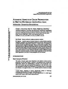
FIG. 1: The geometry of the model. We consider a cubic lattice of conducting bonds with a weak plane in the middle where we place fuses with random breaking threshold. A notch of lenghth a is placed in the weak plane at the beginning of the simulation. The voltage drop is either applied between the top and bottom planes (plane loading) or at the left edges of the plates, on the dotted lines (line loading).

II.

THE MODEL

Here we consider crack propagation under antiplane deformation, a scalar problem that can be mapped to an electrical analog: the random fuse model (RFM). In the RFM [32] a set of conducting bonds, with unit conductivity σ0 = 1, are arranged on a cubic lattice of size L × L × H. To simulate the presence of a weak plane, the vertical bonds crossing the central horizontal plane are replaced by fuses. When the local current ij overcomes a randomly chosen threshold tj , the fuse burns irreversibly. The thresholds are randomly distributed based on a thresholds probability distribution, p(t). In addition, an edge notch is placed on one side of the weak plane. Periodic boundary conditions are imposed in the direction parallel to the notch to simulate an infinite sys-

tem and a constant voltage difference, V , is applied between the top and the bottom plates of the lattice (plane loading) or between two edges (line loading). See Fig. 1 for an illustration of the geometry. The second boundary condition resembles the loading applied in experiments, although here we consider mode III (antiplane shear) while the experiments where performed under mode I (tension). Numerically, we set a unit voltage difference, V = 1, and solve the Kirchhoff equations to determine the current flowing in each of the fuses. Subsequently, for each fuse j, the ratio between the current ij and the breaking threshold tj is evaluated, and the bond jc having the i largest value, maxj tjj , is irreversibly removed (burnt). The current is redistributed instantaneously after a fuse is burnt implying that the current relaxation in the lattice system is much faster than the breaking of a fuse. Each time a fuse is burnt, it is necessary to re-calculate the current redistribution in the lattice to determine the subsequent breaking of a bond. The process of breaking of a bond, one at a time, is repeated until the lattice system falls apart. In this work, we assume that the bond breaking thresholds are distributed based on a uniform probability distribution, which is constant between 0 and 1. An alternative would be to study power law distributions exponents and control the disorder strength varying the exponent, as done in Ref. [33]. Since the robustness of the model behavior with respect of disorder has been extensively studied in the literature we concentrate our effort on a single type of disorder, extending the statistical sampling and the range of lattice sizes. Numerical simulation of fracture using large fuse networks is often hampered due to the high computational cost associated with solving a new large set of linear equations every time a new lattice bond is broken. Although the sparse direct solvers presented in [34] are superior to iterative solvers in two-dimensional lattice systems, for 3D lattice systems, the memory demands brought about by the amount of fill-in during the sparse Cholesky factorization favor iterative solvers. The authors have developed an algorithm based on a block-circulant preconditioned conjugate gradient (CG) iterative scheme [35] for simulating 3D random fuse networks. The blockcirculant preconditioner was shown to be superior compared with the optimal point-circulant preconditioner for simulating 3D random fuse networks [35]. Since these block-circulant and optimal point-circulant preconditioners achieve favorable clustering of eigenvalues, these algorithms significantly reduced the computational time required for solving large lattice systems in comparison with the Fourier accelerated iterative schemes used for modeling lattice breakdown [33, 36]. Using the algorithm presented in [35], we have performed numerical simulations on 3D cube lattice networks with L = 100 and H varying from 6 to 100.

3 III.

ELASTIC INTERACTIONS AND CRACK FRONT STABILITY

1

Unstable 0.8

0.6

a/L

Before studying planar crack propagation, it is instructive to study how the stress is distributed in presence of a crack of length a in a sample of thickness H considering the two boundary conditions employed. An analysis of the stress concentration is useful to assess the stability of the crack under a constant applied voltage. To this end we define an enhancement factor K ≡ Va /V , where Va is the voltage drop across the vertical bonds ahead of a crack of length a under an applied voltage V . Notice that the enhancement factor K is a discrete version of the stress intensity factor usually defined in the continuum to quantify the divergence of the stress ahead of the crack tip. Here, we are working with a discrete lattice and therefore do not have to worry about singularities. Another important difference is that since we are simulating the system imposing a voltage drop (or displacement), we define K in terms of voltages rather than currents.

relative thickness H/L using the two different boundary conditions. From this graph one can define the regions of crack stability by considering the conditions for which K decreases with a. In this way, we see that under plane loading cracks are never stable although for small H/L, we observe a region of marginal stability where K is roughly constant. On the other hand, under line loading K decreases exponentially for small H/L, leading to stable crack propagation. Notice however, that for larger H/L, at small and large a, we would still expect unstable crack growth. The observations can be summarized in a phase diagram, Fig. 3, where we report the stable and unstable crack growth regions for line loading.

0.1

Stable crack growth 0.4

0.01

K

0.2

0.001

Unstable H=10 H=20 H=30 H=40 H=50 H=60 H=70 H=80 H=90 H=100

0.0001

1e-05

K

0.1

0.01

0

0.2

0.4

0.6

0.8

1

a/L

FIG. 2: The factor K as a function of the crack length, computed numerically for systems with different thickness H. Here, K is defined as the voltage drop in the bonds ahead of the crack tip for unit applied voltage. In the top panel, the system is loaded by imposing a constant voltage at the left edges of the system (line loading). In the bottom panel, the constant voltage is imposed on the entire top plate (plane loading).

To link K to the crack stability, we consider its variation as a function of the crack length a. If K increases with a we expect, on average, an unstable crack growth. This is because as the crack advances by one step the voltage drop ahead of it increases making a further failure more likely. This is of course rigorously true for only for very weak disorder and occasionally one can find a stable crack even when K increases, due to a particular combination of the random thresholds. In Fig. 2 we report K as a function of a for different values of the

0

0

0.2

0.4

0.6

0.8

1

H/L

FIG. 3: The phase diagram of the crack under line loading. The stable region is defined by a decrease of K as a is increased, implying that the stress in front of the crack decreases as the crack advances. Under plane loading the crack is always unstable or at most marginally stable (i.e. K = const).

According to continuum theory in the limit H → √ ∞, the current ahead of the crack should decay as 1/ r. For finite thickness we expect that a characteristic length emerges [28]. As shown in Fig 4, the current is found to decay exponentially defining a characteristic length ξ. Under line loading, the current decays to zero, while for plane loading it decays to a value i∞ that decreases as 1/H, vanishing as H → ∞ (see the inset of Fig 4b). Deviations from the exponential behavior can be seen at short distances and large H, showing that the decay is √ crossing over to the expected 1/ r behavior. Since we are interested in planar crack propagation in presence of disorder, we study the variations in the enhancement factor due to a small variation in the crack profile. We consider a straight planar crack of length a = 8 and remove a single fuse ahead of the crack. We then compute the increment J(x) of the enhancement factor K as a function of the distance from the removed fuse. This function is closely related to the first-order variation of the stress intensity factors, computed by Gao and Rice [37] and commonly employed in line models for planar crack front propagation [12–14]. Based on this analogy, we can expect that in the limit H → ∞ it

4 100

50 (a)

40

H=4 H=10 H=20 H=36 H=50 H=70 H=100 -1/2 x

0.01

10

40

0.1

H=4 H=10 H=20 H=36 H=50 H=70 H=100 -2 y

(a)

ξ

30

line plane

20

1

10 0

0

20

60

80

100

Cξ J(y)

I(x)

0.1

H

0.01 0.001

0.001

0.0001 1e-05

0

20

40

0.8

x

80

60

1e-06 0.01

100

0.1

1

10

100

y/ξ||

1 (b)

0.6

H=4 H=10 H=20 H=36 H=50 H=70 H=100 -2 y

10000

0.1

100

0.01

10

12

100

H

0.4

CξJ(y)

I(x)

0.5

b)

Ioo

H=4 H=10 H=20 H=36 H=50 H=70 H=100

0.7

8 ξ||

0.3

10 1

0.01

0.2

6 4 line plane

2

0.1

0 0.0001

0

0

20

40

x

60

80

0

10

20

30 H

40

50

60

100 0.01

0.1

1

10

100

y/ξ||

FIG. 4: The vertical current across the weak plane decays exponentially as a function of the distance from the crack tip for different thicknesses for both line and plane loading. (a) For line loading, the current decays exponentially to zero. A characteristic length ξ can be extracted from the decay of the currents. As shown in the inset, ξ is a linear function of the thickness H, but it is larger for line loading (i.e. ξline ≃ 3ξplane ) (b) For plane loading, the current decays exponentially until it reaches a constant value, which decreases as 1/H (inset)

FIG. 5: The variations in the stress intensity factor following the failure of one bond ahead of the crack as a function of the distance from the bond parallel to the crack direction. This is equivalent to a self-interaction kernel, scaling as 1/y 2 up to a cutoff length ξk . Data for different thickness are collapsed by rescaling the distance by a characteristic length ξk whose values are reported in the insets. Results for line loading (a) and plane loading (b).

IV.

should be J(x) ∝ x−2 [37]. This results is confirmed by our simulations, reported in Fig. 5, showing that the a finite thickness H induces again a characteristic length ξ|| . The data obtained for different H can be collapsed according to the scaling form J(x) = x−2 f (x/ξ|| ), where f (x) decays exponentially and ξ|| is obtained from a fit. In the case of plane loading, we find that ξ|| depends on H and goes linearly to zero as H → 0. For line loading, however, the characteristic length ξ|| depends also on the crack size a and therefore it does not go to zero as H → 0 (see Fig 6)

CRACK FRONT ROUGHNESS AND AVALANCHES

As we load the system, the crack advances but due to the presence of disorder in the breaking thresholds the crack front roughens and dynamics is composed by a sequence of avalanches (Fig. 6), in close analogy to what is observed in experiments [21–25, 27]. To quantify the fluctuations in the crack morphology as a function of the sample thickness, we follow the multiscaling analysis commonly employed to study fracture fronts [27, 38–40] and compute the q−moments of the correlation function Cq (x) = (hh(x′ + x)h(x′ )i)1/q ,

(1)

where h(x) is the position of the front. We perform the average over different realizations of disorder and consider only cracks located in the central part of the lattice, to avoid boundary effects. The results are illustrated in Fig 7 where we show that for large thickness (i.e. a cubic system with H = L) all the moments scales as xζ , with

5

Cq(x)/Cq(L/2)

1

q=1 q=2 q=3 q=4 q=5 0.1

1

10

100

x

Cq(x)/Cq(L/2)

1

FIG. 6: The avalanche progression as a function of the loading model and the sample thickness. Different avalanches are identified by random colors.

ζ ≃ 0.33 on large length scales and an indication of multiscaling behavior at small lengthscales (Fig 7a). This is very similar to what is found in experiments [27]. At low thicknesses, however, we observe a wide multiscaling regime over all the available lengthscales (Fig 7b). This result indicates that the sample thickness controls the crossover scale between the short-scale multiscaling regime and the large-scale interface depinning scaling. The nature and morphology of the avalanches depends on the loading mode and the thickness as shown in Fig. 6. Under line loading and for a small thickness, crack line motion is hindered by a strong restoring force which limits the avalanche size. For a large thickness and for plane loading, the front dynamics is unstable and therefore we observe large avalanches that span a considerable fraction of the system together with other smaller avalanches. The progression of the avalanches can be observed in Fig 8 where we report the total lattice damage D, defined as the number of broken bonds, for typical realizations of the simulations. D illustrates nicely the effect of the stability analysis from above on avalanches. Under line loading and low thickness, we observe a sequence of random avalanches with wide size distribution. For larger thickness, we observed the nucleation of large avalanches which correspond to unstable crack growth (see Fig 8a). The role of instability is even more apparent under plane loading we see large system spanning avalanches (see Fig 8b). The distribution of avalanche sizes for line loading is reported in Fig. 9. For small and intermediate thickness we observe a power law distribution with exponent

q=1 q=2 q=3 q=4 q=5 ζ=0.33

1

10

x

100

FIG. 7: The q− moments of the correlation functions for cracks under plane loading for H=6 (top) and H=100 (bottom). The dashed line indicates a power law with exponent ζ = 0.33.

τ ≃ 1.25 and a cutoff that increases with the thickness. The measured exponent is in agreement with the result expected for the crack line depinning model [15, 16]. For larger thickness, we see a deviation from this result and the power law exponent becomes much larger (τ ≃ 2) and the distribution displays a peak at large avalanches which is a signature again of the large unstable avalanches.

V.

STRENGTH DISTRIBUTION AND SIZE EFFECTS

In Fig. 10 we report the voltage-current curves obtained in the model under planar loading for different thickness values. These curves are related to the stress strain curves by defining shear stress as σ ≡ I/L2 and shear strain as ǫ ≡ V /H. The inset of Fig. 10 displays the size effect for plane and line loading. While for plane loading the strength decreases with the thickness, for line loading the strength increases at large thickness. This crossover is due to the fact that the planar crack becomes unstable at larger H as also illustrated in Fig. 8. We also measure the stress survival distribution S(σ) defined as the probability that the sample does not frac-

6 3000

a)

H=6 H=10 H=20 H=36 H=50 H=70 H=100

8000

6000

H=10 H=20 H=50 H=100

2500

2000 4000 plane loading line loading

I

D

3500 1500

3000 Ic

4000 1000

2500 2000

2000

1500 500

1000

0

20

40

80

60

100

H

0

0

10

5

15

20

0

30

25

V

0.1

0.2

b) H=10 H=20 H=50 H=100

0.4

0.5

1

4000

a)

H=10 H=20 H=50 H=100 (1-erf(x))/2

0.8

D

0.3 V

FIG. 10: The voltage-current curve for the model under plane loading. The inset shows the fracture current as a function of the thickness H for plane and line loading.

6000

5000

0

3000

H=6 H=10 H=20 H=36 H=50 H=70 H=100 (1-erf(x))/2

b)

0.6

S(σ)

2000

1000

0

0.4

0

2

4

8

6

0.2

V

FIG. 8: The accumulated damage as a function of the applied voltage for a) line loading and b) plane loading. The staircase character of the curve is a signature of avalanche behavior.

H=6 H=10 H=20 H=36 H=50 H=70 H=100 τ=1.25

P(s) 1e-06

10

100

s

1000

-1

0

1

2

(σ−)/SD

VI.

0.0001

1

-2

3

-2

-1

0

1

2

(σ−)/SD

3

FIG. 11: The stress survival distribution for a) plane and b) line loading as a function for the sample thickness. Data are plotted as a function of reduced variables (σ − hσi)/SD and the corresponding Gaussian distribution is reported for comparison.

1

0.01

0 -3

10000

FIG. 9: The avalanche size distribution measured under line loading for different values of the sample thickness.

ture at stress σ. In both cases the distribution is well described by Gaussian statistics as it is shown in Fig. 11 by using reduced variables (σ − hσi)/SD, where hσi and SD are the average and standard deviation of σ. The presence of Gaussian statistics is expected in systems that have one dominating crack so that statistical size effects described by extreme value theory are not present [41].

CONCLUSIONS

Planar crack propagation has been for some time a test ground for theories of depinning in the context of fracture, and much progress has been made. For understanding the connections between the paradigm of a non-equilibrium critical point for a driven crack and actual behavior in an experiment, it is necessary to investigate in a general manner the effects of loading conditions and sample geometry. Usual theory accounts for the distance the crack propagates, and for the finite length of the crack line and provides predictions. Here, we have added the effect of the finite sample thickness, which influences among others the effective form of the interactions along the crack (”elastic kernel”). The loading has also been found to be of importance, and the comparison between the line and plane loading cases, where the former is close to most recent experiments, in fact shows major differences. The coarsegrained stability properties of the ”experiment” are decisive for the presence of the collective phenomena, ie.

7 avalanches. We would think that this hints of a need for further investigations of other possible loading protocols. Generally, we find also the signatures of the universality class of long-range elastic line depinning: avalanches with the expected size distribution, and line roughening with a roughness exponent as expected. These observations should have also an impact on understanding the design of interfacial layers for adhesive properties or for fracture toughness.

visiting professor program of Aalto University, School of Science and the Aalto Science Institute. MJA thanks the support from the Academy of Finland through the COMP Center of Excellence. Part of this work was performed when PKVVN was a senior researcher at Oak Ridge National Laboratory. PKVVN acknowledges the support received from the Mathematical, Information and Computational Sciences Division, Office of Advanced Scientific Computing Research, U.S. Department of Energy under Contract No. DE-AC05-00OR22725 with UTBattelle,LLC.

Acknowledgments

SZ is supported by the European Research Council Advanced Grant 2011 - SIZEFFECTS and thanks the

http://link.aip.org/link/?APL/88/061912/1. [1] M. J. Alava, P. Nukala, and S. Zapperi, Adv. Phys. 55, [21] J. Schmittbuhl and K. J. Maloy, Phys. Rev. Lett. 78, 349 (2006). 3888 (1997). [2] I. C. van den Born, A. Santen, H. D. Hoekstra, and J. T. [22] A. Delaplace, J. Schmittbuhl, and K. J. Maloy, Phys. M. D. Hosson, Phys. Rev. B 43, R3794 (1991). Rev. E 60, 1337 (1999). [3] Z. P. Bazant, Arch. Appl. Mech. 69, 703 (1999). [23] K. J. Maloy and J. Schmittbuhl, Phys. Rev. Lett. 87, [4] L. Sutherland, R. Shenoi, and S. Lewis, Composite Sci. 105502 (2001). Techn. 209, 1999 (1999). [24] K. J. Maloy, J. Schmittbuhl, A. Hansen, and G. G. Ba[5] B. B. Mandelbrot, D. E. Passoja, and A. J. Paullay, Natrouni, International Journal of Fracture 121, 9 (2003). ture 308, 721 (1984). [25] K. J. Maloy, S. Santucci, J. Schmittbuhl, and R. Tous[6] E. Bouchaud, Journal of Physics: Condensed Matter 9, saint, Phys. Rev. Lett. 96, 045501 (2006). 4319 (1997). [26] L. I. Salminen, J. M. Pulakka, J. Rosti, M. J. Alava, and [7] D. Bonamy and E. Bouchaud, Physics ReK. J. Niskanen, Europhys. Lett. 73, 55 (2006). ports 498, 1 (2011), ISSN 0370-1573, URL [27] S. Santucci, M. Grob, R. Toussaint, J. Schmithttp://www.sciencedirect.com/science/article/pii/S0370157310002115. tbuhl, A. Hansen, and K. J. Maly, EPL (Eu[8] L. Ponson, D. Bonamy, and E. Bouchaud, Phys. Rev. rophysics Letters) 92, 44001 (2010), URL Lett. 96, 035506 (2006). http://stacks.iop.org/0295-5075/92/i=4/a=44001. [9] D. Bonamy, L. Ponson, S. Prades, E. Bouchaud, and [28] S. Zapperi, H. J. Herrmann, and S. Roux, Eur. Phys. J. C. Guillot, Phys. Rev. Lett. 97, 135504 (2006), URL http://link.aps.org/doi/10.1103/PhysRevLett.97.135504. B 17, 131 (2000). [29] M. Zaiser, P. Moretti, A. Konstantinidis, and E. C. [10] J. P. Bouchaud, E. Bouchaud, G. Lapasset, and Aifantis, Journal of Statistical Mechanics: TheJ. Plan`es, Phys. Rev. Lett. 71, 2240 (1993). ory and Experiment 2009, P11009 (2009), URL [11] P. Daguier, B. Nghiem, E. Bouchaud, and F. Creuzet, http://stacks.iop.org/1742-5468/2009/i=11/a=P11009. Phys. Rev. Lett. 78, 1062 (1997). [30] J. Schmittbuhl, A. Hansen, and G. G. Batrouni, Phys. [12] J. Schmittbuhl, S. Roux, J. P. Villotte, and K. J. Maloy, Rev. Lett. 90, 045505 (2003). Phys. Rev. Lett. 74, 1787 (1995). [31] A. Stormo, K. S. Gjerden, and A. Hansen, [13] S. Ramanathan and D. S. Fisher, Phys. Rev. Lett. 79, Phys. Rev. E 86, 025101 (2012), URL 877 (1997). http://link.aps.org/doi/10.1103/PhysRevE.86.025101. [14] S. Ramanathan and D. S. Fisher, Phys. Rev. B 58, 6026 [32] L. de Arcangelis, S. Redner, and H. J. Herrmann, Journal (1998). of Physics (Paris) Letters 46(13), 585 (1985). [15] D. Bonamy, S. Santucci, and L. Ponson, Physical Review [33] G. G. Batrouni and A. Hansen, Physical Review Letters Letters 101, 045501 (pages 4) (2008). 80, 325 (1998). [16] L. Laurson, S. Santucci, and S. Zapperi, [34] P. K. V. V. Nukala and S. Simunovic, J. Phys. A: Math. Phys. Rev. E 81, 046116 (2010), URL Gen. 36, 11403 (2003). http://link.aps.org/doi/10.1103/PhysRevE.81.046116. [35] P. K. V. V. Nukala and S. Simunovic, J. Phys. A: Math. [17] L. Laurson and S. Zapperi, Journal of Statistical MechanGen. 37, 2093 (2004). ics: Theory and Experiment 2010, P11014 (2010), URL http://stacks.iop.org/1742-5468/2010/i=11/a=P11014. [36] T. Ramstad, J. . H. Bakke, J. Bjelland, T. Stranden, and A. Hansen, Phys. Rev. E 70, 036123 (2004). [18] D. Ertas and M. Kardar, Phys. Rev. E 49, R2532 (1994). [37] H. Gao and J. R. Rice, J. Appl. Mech. 56, 828 (1989). [19] A. Rosso and W. Krauth, Phys. Rev. E 65, 025101 [38] E. Bouchbinder, I. Procaccia, S. Santucci, and (2002). L. Vanel, Phys. Rev. Lett. 96, 055509 (2006), URL [20] W. P. Vellinga, R. Timmerman, R. van Tihttp://link.aps.org/doi/10.1103/PhysRevLett.96.055509. jum, and J. T. M. D. Hosson, Applied Physics [39] M. J. Alava and K. J. Niskanen, Rep. Prog. Phys. 66, Letters 88, 061912 (pages 3) (2006), URL

8 [41] M. J. Alava, P. K. V. V. Nukala, and S. Zapperi, Journal 669 (2006). of Physics D: Applied Physics 42, 214012 (2009), URL [40] S. Santucci, K. J. M˚ aløy, A. Delaplace, J. Mathiesen, http://stacks.iop.org/0022-3727/42/i=21/a=214012. A. Hansen, J. O. Haavig Bakke, J. Schmittbuhl, L. Vanel, and P. Ray, Phys. Rev. E 75, 016104 (2007), URL http://link.aps.org/doi/10.1103/PhysRevE.75.016104.