Rotation-Invariant Texture Retrieval via Signature Alignment based on Steerable sub-Gaussian Modeling George Tzagkarakis∗ 1 , Baltasar Beferull-Lozano2 , Associate Member, IEEE, and Panagiotis Tsakalides1 , Member, IEEE
1
Department of Computer Science, University of Crete & Institute of Computer Science - FO.R.T.H.
ICS-FORTH, P.O. Box 1385, 711 10 Heraklion, Crete, Greece Phone: +30 2810 391670, Fax: +30.81 - 391601 E-mail:
[email protected],
[email protected]
2
”Group of Information and Communication Systems”
Instituto de Rob´otica - Escuela T´ecnica Superior de Ingenier´ıa Universidad de Valencia Pol´ıgono de La Coma, s/n 46071, P.O. Box: 2085 Valencia, SPAIN E-mail:
[email protected]
Submitted to: IEEE Trans. on Image Processing (November 2006) EDICS: 5-OTHE
1
Abstract This paper addresses the construction of a novel efficient rotation-invariant texture retrieval method that is based on the alignment in angle of signatures obtained via a steerable sub-Gaussian model. In our proposed scheme, we first construct a steerable multivariate sub-Gaussian model, where the fractional lower-order moments (FLOMs) of a given image, are associated with those of its rotated versions. The feature extraction step consists of estimating the so-called covariations between the orientation subbands of the corresponding steerable pyramid at the same or at adjacent decomposition levels and building an appropriate signature that can be rotated directly without the need of rotating the image and recalculating the signature. The similarity measurement between two images is performed using a matrix-based norm that includes a signature alignment in angle between the images being compared, achieving in this way the desired rotation-invariance property. Our experimental results show how this retrieval scheme achieves a lower average retrieval error, as compared to the previously proposed methods having a similar computational complexity, while at the same time being competitive with the best currently known stateof-the-art retrieval system. In conclusion, our retrieval method provides the best compromise between complexity and average retrieval performance.
Index Terms Rotation-invariant texture retrieval, fractional lower-order moments, steerable multivariate sub-Gaussian model.
I. I NTRODUCTION Increasing accumulation of visual information in large digital databases has been prominent during the last decades. To improve the management of these collections, it is necessary to have effective and precise methods to search and interact with them. For this purpose, content-based image retrieval (CBIR) from unannotated image databases has gained an important interest in the research community. CBIR is a set of techniques for retrieving relevant images on the basis of automatically derived features, which accurately specify the information content of a given image. There exist several practical examples where a CBIR plays a major role. Two typical examples are: a) retrieval of images (through the Internet) that are similar to a given query image, b) remote satellite sensing of images where only novel images have to be transmitted and where the novelty is checked on the earth by performing a comparison between the features of a query and the features of images contained in a database.
2
In a typical CBIR system we can distinguish two major tasks, namely feature extraction (FE) and similarity measurement (SM). In the FE step, a set of features, constituting the so-called image signature, is generated after an image transformation, to accurately represent the content of a given image. In order to guarantee the computational efficiency of the retrieval process1 , this set has to be much smaller in size than the original image, while capturing as much as possible the important information from the image, for the purpose of classification. During the SM step, a distance-like function is usually employed, which measures how close each image, from the database, is to a given query image, by measuring the distance between their corresponding signatures. Typical low-level image features, such as color [1], shape [2] and texture [3], are commonly used in CBIR applications. In this work, we focus on the use of texture information for the description of image content. Loosely speaking, the class of texture images includes images that are spatially homogeneous and consist of repeated elements (image texels), often subject to some randomization in their location, size, color, and orientation. However, it is also important to mention that even though this assumption of homogeneity is done, our experimental results show that our method also tolerates certain degree of non-homogeneity. Several previously developed texture extraction methods make use of multi-orientation filter-banks and spatial Gabor filters [4]. The basic assumption for these approaches is that the energy distribution in the frequency domain identifies a texture. These retrieval systems use as similarity measures simple norm-based distances (e.g. Euclidean distance) on the extracted image signatures. The design of retrieval systems in a transform-domain is justified by the observation that often a linear, invertible transform results in a set of coefficients whose structure is simpler to model than the structure of the original image in the pixel-domain. Features such as oriented edges, ridges and lines, are prominent in real-world images. For such images, the 2-dimensional wavelet transform is a powerful modeling tool, providing a natural arrangement of the wavelet transform coefficients into multiple scales and oriented subbands representing the edges in different directions [5]. In previous works, the texture information has been modeled using the first or second-order statistics of the coefficients obtained via a Gabor wavelet transform [6], or an overcomplete wavelet decomposition constituting a tight frame [7]. Moreover, only until recently, the wavelet coefficients have been modeled either as independent Gaussian variables, or as jointly Gaussian vectors [8]. In the texture retrieval scheme proposed in this work, the task of FE is considered in a statistical 1
In other cases, where the encoder and decoder are physically separated, a reduction in the necessary transmission bandwidth
is also a very important requirement.
3
framework. In particular, the signature of a given image contains the estimations of fractional lowerorder moments (FLOMs) between the orientation subbands at the same or at adjacent decomposition levels. This is justified by the observation that the wavelet transforms of real-world images tend to be sparse, that is, they result in a large number of small amplitude coefficients and a small number of large amplitude coefficients [9]. This property gives rise to peaky and heavy-tailed non-Gaussian marginal distributions of the wavelet subband coefficients, whose statistics are best described by lower than secondorder moments [9], [10], as opposed to the traditional Gaussian modeling. The SM step employs an appropriate norm-based distance function that exploits the heavy-tailed behavior of the distributions of the transform coefficients. In previous work [9], [11], experimental results have proven that the generalized Gaussian density (GGD) is a good member of the class of non-Gaussian distributions for modeling the marginal behavior of the wavelet coefficients. Recently, GGD models have been also introduced in a statistical framework for texture retrieval in CBIR applications, by jointly considering the two problems of FE and SM [12]. On the other hand, in recent work [13], we have shown that an improved description of the texture information can be achieved if we take into consideration the actual heavy-tailed behavior of the distribution of transform coefficients. We demonstrated that successful modeling of subband decompositions of many texture images is achieved by means of Symmetric alpha-Stable (SαS ) marginal distributions [14], [15], which very often provide a better fit than the generalized Gaussian distribution (GGD) for heavy-tailed data. After extracting the SαS model parameters, we analytically derived the Kullback-Leibler Divergence (KLD) between two SαS distributions. Our formulation improved the retrieval performance, resulting in a decreased average retrieval error for images with distinct non-Gaussian statistics, compared with the GGD model [16]. This motivated the statistical model in our work in this paper, where we use a joint (multivariate) SαS distribution model. Only quite recently, several CBIR approaches have taken into account the important interdependencies between different (transform) subbands of a given image, which can be employed in order to provide a more accurate representation of the texture image profile. For instance, Huang studied the correlation properties of wavelet transform coefficients at different resolution levels and different subbands within each level, applying these properties on an image coding scheme based on neural networks [17]. Portilla and Simoncelli developed an improved algorithm for synthesizing texture images by setting different constraints on the correlation between the transform coefficients and their magnitudes [18]. On the other hand, the theory of Markov random fields has enabled a new generation of statistical texture models, taking into account possible interdependencies between the transform coefficients, in
4
which the full model is characterized by statistical interactions within local neighborhoods [19]. Similarly, a new framework for statistical signal processing based on wavelet-domain Hidden Markov Models was proposed in [20]. It provides an attractive modeling of both the non-Gaussian statistics and the property of persistence across scales in a wavelet decomposition. In this paper, we exploit transform-domain interdependencies by tying up the subband coefficients at adjacent orientations and/or scales in vectors, which are then considered to be drawn from a multivariate sub-Gaussian distribution. Within the sub-Gaussian framework, we use the notion of covariation, that is, fractional lower-order statistics, instead of the second-order covariance, in order to describe the interdependencies between wavelet coefficients at different image orientations and scales. The joint subGaussian modeling preserves the heavy-tailed behavior of the marginal distributions, as well as the strong statistical dependence across orientations and scales. An important desirable property of a CBIR system is rotation invariance. This is an issue that has been previously pursued by various researchers. Greenspan et al. [21], Haley and Manjunath [22], [23] employed rotation-invariant structural features, using autocorrelation and Discrete Fourier Transform (DFT) magnitudes, obtained via multiresolution Gabor filtering. Recently, a rotation-invariant texture retrieval system based on steerable pyramids was proposed by Beferull-Lozano et al. [24], where the correlation matrices between several basic orientation subbands at each level of a wavelet pyramid are chosen as the energy-based texture features. Do and Vetterli [25] derived a steerable rotation-invariant statistical model for texture description, by enhancing a recently introduced technique based on a waveletdomain Hidden Markov Model (HMM) [20]. Liu and Picard [26] exploited the effectiveness of the 2dimensional Wold decomposition of homogeneous random fields, in order to extract features that represent perceptual properties described as “periodicity”, “directionality” and “randomness”. In recent work [16], we designed an efficient rotation-invariant texture retrieval system by applying a joint sub-Gaussian model on a steerable pyramid decomposition [27] of the images, followed by a Gaussianization process, resulting in a set of (modified) pyramid subbands whose coefficients are almost jointly Gaussian. Then, the SM was carried out by constructing a rotation-invariant version of the KLD between multivariate Gaussian density functions, describing statistically the Gaussianized subbands. Although the method described in [16] results in an increased retrieval performance, compared with the previously developed methods based on second-order statistics, a main drawback is its computational complexity due to the Gaussianization procedure, since it involves the use of a sufficiently large neighborhood for each transform coefficient and repeating this procedure across all the pyramid. In return, in this work we propose a rotation-invariant texture retrieval system with reduced computational complexity,
5
by constructing directly a steerable multivariate sub-Gaussian model and then by applying a rotationinvariant deterministic similarity function based on matrix norms, similar to the one described in [24], while at the same time providing an average retrieval performance which is superior to the current stateof-the-art methods with similar complexity (e.g. [24], [25]), and being at the same time competitive with the current best method [16], which has, on the other hand, a much higher computational cost than the retrieval method we present here. Following the retrieval method presented in this paper, we avoid the computational burden introduced by the Gaussianization procedure during the FE step, while maintaining a very similar average retrieval error to the one in [16]. The rest of the paper is organized as follows: in Section II, we develop a rotation-invariant texture retrieval system based on a steerable multivariate sub-Gaussian model, which exploits the non-Gaussian behavior of the marginal and joint distributions of the subband coefficients obtained via a steerable pyramid decomposition. In Section III, we apply our scheme to a set of real-world textures in order to evaluate its retrieval performance and we compare it with the performance of other recently introduced texture retrieval techniques. Finally, we draw several conclusions and explore avenues of future research in Section IV. II. ROTATION -I NVARIANCE VIA A S TEERABLE M ULTIVARIATE SUB -G AUSSIAN M ODEL A desirable property of any texture retrieval system is rotation invariance. Consider, for instance, the case of a content-based search over the Internet, where we are interested in retrieving images containing the same object with the one of a given query and the orientation of this object can vary among the images, or the case of remote satellite sensing, where there could be different rotated versions of the same area of interest. Many approaches for texture retrieval make use of transforms which suffer from rotation and translation variance. The standard wavelet transform, used in the previously developed retrieval methods, belongs in this class of transforms, that is, it lacks the properties of translation and rotation invariance. This results in a mismatch of the retrieval process when the image orientation varies. In fact, the wavelet coefficients of a rotated version will be completely different, in the sense that they will not be simply rotated versions of the wavelet coefficients of its original version. A way to overcome this problem is to replace the standard wavelet transform with a steerable pyramid [27], [28], which is a linear, multi-scale, multi-orientation image decomposition produced by a set of orientation filters, generated by a set of basis functions (directional derivative operators). Steerable pyramids are overcomplete and possess the desired properties of rotation invariance and (approximate) translation invariance.
6
In this section, we design a texture retrieval technique that performs an angular alignment between texture images, thus, achieving (indirectly) the rotation-invariance property. This technique is based on the joint sub-Gaussian modeling of several coefficients obtained from a steerable pyramid, defining features that incorporate dependence across orientations and scales2 . In particular, we construct a steerable model, relating the fractional lower-order statistics of a rotated image with that of its original version and then we derive a rotation-invariant similarity function. The development of steerable model implies extracting features which are “steerable”, that is, given the features of an image, we should be able to obtain the features corresponding to the same image rotated at an angle θ, without having to re-extract the features from the rotated image3 . The use of the family of multivariate sub-Gaussian distributions, as an accurate tool for modeling the heavy-tailed behavior of the steerable pyramid coefficients, has been justified in [16], showing that it provides a statistical description that is more complete to both Gaussian and generalized Gaussian distributions, which have been used in previous texture retrieval techniques [25]. On the one hand, the oriented subbands of a steerable pyramid obtained from a texture image exhibit various degrees of non-Gaussianity both marginally and as joint distributions. On the other hand, the joint modeling of coefficients at adjacent orientations and scales via a multivariate sub-Gaussian model is motivated by several previous studies on their correlation properties [17] and the fact that the components of a joint sub-Gaussian random vector, corresponding to these coefficients, are by definition highly dependent [14]. Before providing the definition of a sub-Gaussian random vector, we introduce first briefly the family of α-Stable distributions. The α-Stable distribution is best defined by its characteristic function [29]: ³ ¡ ¢´ exp ıδt − γ α |t|α 1 − ıβ(sign t) tan πα , α 6= 1 2 ϕ(t) = (1) ³ ´ ¡ ¢ exp ıδt − γ|t| 1 + ıβ 2 (sign t) ln |t| , α = 1 π where sign t = {1 if t > 0, 0 if t = 0, −1 if t < 0}. The α-Stable distribution is characterized by four parameters: α is the characteristic exponent, taking values 0 < α ≤ 2, δ (−∞ < δ < ∞) is the location parameter, γ (γ > 0) is the dispersion of the distribution and β (−1 ≤ β ≤ 1) is the index of skewness. The characteristic exponent is a shape parameter, which controls the “thickness” of the tails of the density function. The smaller the α, the heavier the tails of the α-Stable density function. The dispersion parameter determines the spread of the distribution around its location parameter, similar to the 2
In the following, we will often refer to the “orientation” and “scale” with their equivalent terms “subband” and “level”,
respectively. 3
Through the next sections, we consider counter-clockwise rotation.
7
variance of the Gaussian. We will denote α-Stable distributions by Sα (γ, β, δ) and write X ∼ Sα (γ, β, δ) to indicate that X is a random variable that follows an α-Stable distribution with parameters (α, γ, β, δ). A random variable X is said to follow a Symmetric alpha-Stable (SαS ) distribution if and only if β = δ = 0. A SαS distribution is called standard if γ = 1 and δ = 0. A SαS distribution is best defined
by its characteristic function given by the following expression: ϕ(t) = exp(−γ α |t|α ),
(2)
In general, no closed-form expressions exist for most SαS density and distribution functions. Two important special cases of SαS densities with closed-form expressions are the Gaussian (α = 2) and the Cauchy (α = 1). Unlike the Gaussian density, which has exponentially decaying tails, stable densities have tails following an algebraic rate of decay (P (X > x) ∼ Cx−α , as x → ∞, where C is a constant depending on the model parameters), hence random variables following SαS distributions with small α values are highly impulsive. According to the following proposition [14], every SαS random variable is conditionally Gaussian: Proposition 1 ([14]) Let G ∼ Sα0 (γ, 0, 0) with 0 < α0 ≤ 2 and let 0 < α < α0 . Let A be an α/α0 -stable 0
random variable with characteristic function in Laplace form E[exp(−kA)] = exp(−k α/α ), k > 0, i.e. ¡ ¢ 0 πα α0 /α A ∼ Sα/α0 (cos 2α , 1, 0 , and assume G and A to be independent. Then X = A1/α G ∼ Sα (γ, 0, 0), 0) i.e. the random variable X follows a SαS distribution. Proof: In order to prove that the random variable X follows a SαS distribution we have to show that its characteristic function has the form of (2). For any real t we have that the characteristic function of X is given by: £ ¤ 0 0 E[exp(ıtX)] = E[exp(ıtA1/α G)] = E E[exp(ıtA1/α G)]|A (∗)
0
0
= E[exp(−γ α |t|α A)]
(∗∗)
0
0
0
= exp(−(γ α |t|α )α/α ) = exp(−γ α |t|α ),
that is, the characteristic function of X is written in the form of (2), which means that X follows a SαS distribution with characteristic exponent α and dispersion parameter γ . The equation (∗) follows from the fact that G ∼ Sα0 (γ, 0, 0) and thus, its characteristic function is written in the form of (2), while equation (∗∗) follows directly from the assumption about the characteristic function in Laplace form for 0
0
A, by setting k = γ α |t|α .
8
In particular, this implies that if G is a zero-mean Gaussian random variable (i.e. G ∼ S2 (γ, 0, 0)) and if A is a positive α/2-stable random variable independent of G, then X = A1/2 G ∼ Sα (γ, 0, 0), i.e. X is a SαS random variable. Since S2 (γ, 0, 0) = N (0, 2γ 2 ) (= N (E[G], V ar[G])) [14]4 , then any SαS
random variable X ∼ Sα (γ, 0, 0) can be generated as the product of an α/2-stable random variable A, given by Proposition 1 for α0 = 2, and a zero-mean Gaussian random variable G with variance equal to 2γ 2 .
As mentioned above, in our method we are interested in extracting possible interdependencies between pyramid subband coefficients at the same or at adjacent decomposition level. For this purpose, we construct a joint (multivariate) statistical model for the different subbands. A natural way to design this model is to use the result of Proposition 1, that is, that every SαS random variable is conditionally Gaussian. Thus, extending the univariate SαS model (used in our previous work [13]) to a joint (multivariate) model with SαS components (viewed as conditionally Gaussian random variables), leads to the use of the so-called
sub-Gaussian SαS random vector, defined as follows5 [14]: ~ is called a sub-Gaussian SαS random vector (in Rn ) with underlying Gaussian Definition 1 A vector X ~ iff it can be written in the form X ~ = A1/2 G ~ , where A is a positive α -stable random variable with vector G 2 ¡ ¢ πα 2/α ~ parameters A ∼ Sα/2 (cos 4 ) , 1, 0 and G = (G1 , G2 , . . . , Gn ) is a zero-mean Gaussian random
vector, independent of A, with covariance matrix R. A multivariate sub-Gaussian distribution, with underlying covariance matrix R, is often denoted by α-SG(R), where the parameter α is the characteristic exponent, controlling the heaviness of the tails
of the marginal sub-Gaussian distributions. According to Proposition 1, the marginal distributions of the components of a sub-Gaussian vector belong to the family of SαS distributions, namely, the i-th p ~ , Xi ∼ Sα ( V ar(Gi )/2, 0, 0) (where V ar(Gi ) is the variance component of a sub-Gaussian vector X ~ ). As it is described later in this section, of the i-th component of the underlying Gaussian vector G
following our approach, the subband coefficients at adjacent orientations and/or scales, are tied up in vectors which are assumed to be samples of an α-SG(R) distribution. This assumption is also justified in [16]. Since second-order moments do not exist for the family of sub-Gaussian random variables, a quantity called covariation, which plays an analogous role for sub-Gaussian random variables to the one played 4
G ∼ N (µ, σ 2 ) denotes that G is a Gaussian random variable with mean µ and variance σ 2 .
5
In the following, instead of saying sub-Gaussian SαS variable / vector / distribution, we simply use the term sub-Gaussian
variable / vector / distribution.
9
by covariance in Gaussian random variables, has been proposed [14]. Let X and Y be joint sub-Gaussian random variables (representing the coefficients belonging to two different subbands for instance) with αX = αY = α (1 < α ≤ 2), zero location parameters and dispersions γX and γY (γX 6= γY in general),
respectively. Then, for all 1 < p < α, the covariation of X with Y is given by [X, Y ]α =
E{XY } α γY . E{|Y |p }
(3)
In the above expression, we use the notation z
= {z a for z > 0, 0 for z = 0, −(−z)a for z < 0}, for any real number z and a ≥ 0. The covariation coefficient of X with Y is defined by λXY =
[X, Y ]α E{XY } = . [Y, Y ]α E{|Y |p }
(4)
From (4), we observe that we can find an estimation of [X, Y ]α by multiplying an estimated value of λXY and an estimated value of [Y, Y ]α . Since [Y, Y ]α = γYα , an estimation of [Y, Y ]α can be obtained via the Maximum Likelihood (ML) estimation of the characteristic exponent α and the dispersion parameter γY . In the following, we estimate the model parameters (α, γ) using the consistent ML Nolan’s method described in [30], which gives reliable estimates (where the reliability can be evaluated through simulations) and provides the tightest possible confidence intervals. On the other hand, the value of λXY can be estimated directly from (4) by replacing the expectations with sample means, yielding the FLOM estimator [31]: ˆ F LOM = λ
Pn
p−1 sign(Y ) i |Yi | i i=1 X P , n p |Y | i=1 i
(5)
where (Xi , Yi ), i = 1, . . . , n, is a set of independent observations. Our choice of the FLOM estimator is based on its robustness against changes of α and also on the fact that it is very simple and inexpensive to compute. Let the vectors {X~ 1 , X~ 2 , . . . , X~N } constitute a set of N independent realizations of an α-SG(R) distribution, where X~ k = (X k , X k , . . . , X k ), k = 1, . . . , N . The FLOM covariation estimator between 1
2
n
~ is defined by: the i-th and j -th components of the sub-Gaussian vector X PN Xik |Xjk |p−1 sign(Xjk ) α ˆcFijLOM = k=1 P γXj , N k |p |X k=1 j
(6)
where the characteristic exponent α and dispersion parameter γXj are estimated from the set {Xjk }k=1,...,N ˆ to be the matrix with elements using Nolan’s ML estimator. We define the estimated covariation matrix C ˆ ]ij = ˆcF LOM . We can then estimate the elements [R]ij of the underlying covariance matrix, R, using [C ij
the following estimators that we provide in [16]: ¡ ¢2 ˆ ]jj α , ˆ ]jj = 2 α2 [C [R
α
ˆ ]ij = 2 2 [R
ˆ ]ij [C (α−2)
ˆ] 2 [R jj
,
(7)
10
which are both consistent and asymptotically normal6 . Notice that the estimation of covariations and consequently the estimation of the covariation matrices, requires the specification of the parameter p. In [16], we describe a procedure to compute the optimal p as a function of the (estimated) characteristic exponent α, by finding the value of p that minimizes the standard deviation of the covariation estimator (6). For this purpose, we studied the influence of the parameter p on the performance of this estimator via Monte-Carlo simulations, for different values of α > 1. As a general conclusion, the simulations showed that the FLOM covariation estimator approximates accurately the true covariation value and the corresponding value of the optimal p increases as the characteristic exponent α increases. For instance, when α = 1.1, 1.2, 1.3, 1.4, 1.5, the simulations gave the optimal p values to be equal to 0.56, 0.57, 0.59, 0.66 and 0.68, respectively. A steerable pyramid provides a representation that consists of L decomposition levels, where in each level there are J orientation subbands, thus, in total there are L × J subbands. In the following, assume for convenience that the coefficients of an lth-level subband, with dimension N × N , are arranged in a 1 × N 2 row vector by grouping them row-wise. Let Σl and Σlθ denote the sampled correlation matrices, with elements given by the correlations between pairs of subbands, at a given decomposition level l, of the original image I and its rotated version at an angle θ, Iθ , respectively. That is, if we denote by cl (xk , φi ), cl (xk , φj ) the coefficients of the subbands corresponding to the orientations φi , φj (i, j = 1, . . . , J ), placed at the spatial location xk (k = 1, . . . , N 2 ) and level l = 1, . . . , L, then, [Σl ]ij = 1 PN 2 l l l k=1 c (xk , φi )c (xk , φj ). The elements of Σθ are defined similarly. N2 The following proposition states that Σl and Σlθ are equivalent matrices. Proposition 2 ([16], [24]) The relationship between the sampled correlation matrices Σl and Σlθ is given by Σlθ = F(θ)Σl FT (θ),
(8)
ˆ An estimator A(n) (where n is the sample size) is a consistent estimator for a parameter A if: i) Aˆ is asymptotically ˆ ˆ unbiased (i.e. limn→∞ E[A(n)] = A) and ii) its asymptotic variance goes to 0 (i.e. limn→∞ V ar[A(n)] = 0). An estimator ˆ ˆ ˆ A(n) is asymptotically normal if its asymptotic distribution is a Gaussian with mean E[A(∞)] and variance V ar[A(∞)] (i.e. 6
ˆ ˆ ˆ limn→∞ A(n) ∼ N (E[A(∞)], V ar[A(∞)])).
11
where
f1 (φ1 − θ)
f2 (φ1 − θ) · · ·
f1 (φ2 − θ) f2 (φ2 − θ) · · · F(θ) = .. .. .. . . . f1 (φJ − θ) f2 (φJ − θ) · · ·
fJ (φ1 − θ) fJ (φ2 − θ) .. .
,
(9)
fJ (φJ − θ)
with {f1 (·), f2 (·), ..., fJ (·)} being a set of J steering functions. In our work, the J basic angles {φi }i=1,...,J are taken to be equispaced, which makes F(θ) an orthogonal matrix for any angle θ, i.e., FT (θ) = F−1 (θ) (= F(−θ)), and thus, in this particular case, Σl and Σlθ become orthogonally equivalent7 . It
can be easily shown that the above proposition also holds if we consider the sample covariance matrices between the J subbands of a given level l1 and the J subbands of another level l2 . ~ l = [cl (x , φ ), cl (x , φ ), ..., cl (x , φ )]T denote the vector containing the J basic coefficients Let X 1 2 J k k k k at the spatial location xk (k = 1, . . . , N 2 ) and level l = 1, . . . , L. Under a joint sub-Gaussian assumption (this has been justified previously in [16], where it has been found that it gives the best statistical fitting of ~ l are modeled as the marginal and joint distributions of the pyramid subband coefficients), the vectors X k
joint sub-Gaussian vectors
α-SG(Rl ),
with
Rl
denoting the underlying covariance matrix corresponding
to the subbands at the l-th level. Under this assumption, the pyramid coefficients at each subband follow a sub-Gaussian marginal distribution, and thus, the lth-level coefficient at spatial location xk and at any angle θ can be expressed as: cl (xk , θ) =
J X
fi (θ)cl (xk , φi )
i=1
=
J X
¡√ ¢ fi (θ) A clG (xk , φi )
i=1
=
J √ X √ A fi (θ)clG (xk , φi ) = A clG (xk , θ),
(10)
i=1
which means that the pyramid subband coefficients of a rotated image at an angle θ, are also subGaussian random variables with the same characteristic exponent as that of the corresponding subbands of the original (non-rotated) image, and having a Gaussian part which is the rotated version of the original Gaussian part at the same angle θ. This is important because it motivates clearly the construction of a steerable statistical model. 7
Given a matrix A which depends on an angle θ, we use the notations A(θ) and Aθ interchangeably. Following this convention,
we always have that A = A(θ = 0) = Aθ=0 .
12
Let Cl and Clθ denote the covariation matrices with elements that are the estimated covariations between pairs of orientation subbands at the l-th decomposition level of the original image I and its rotated version Iθ , respectively. For instance, the element [Cl ]ij (that is, the estimated covariation between the lth-level subbands corresponding to the orientations φi , φj ) is obtained from (6) by replacing Xik , Xjk
with cl (xk , φi ), cl (xk , φj ), respectively, for k = 1, . . . , N 2 . The elements of Clθ are computed similarly from the subband coefficients of the rotated image Iθ . Notice that the relation between the covariation matrix Cl and the associated underlying covariance matrix Rl is given by (7). This relation is also valid between the elements of the covariation matrix Clθ of the rotated image and the elements of the corresponding underlying covariance matrix Rlθ . Thus, by inverting (7) and expressing the elements of Clθ as a function of the elements of Rlθ , we have: (α−2)/2
α
[Clθ ]ij = 2− 2 [Rlθ ]ij [Rlθ ]jj
.
(11)
Taking into account that Proposition 2 holds for each lth-level, which underlies covariance matrices of the sub-Gaussian model, the replacement of Σl and Σlθ with Rl and Rlθ , respectively in (8), and its combination with (11), yields the following proposition: Proposition 3 Suppose that S = {C1 , C2 , . . . , CL } is the signature obtained from a multivariate sub-Gaussian modeling of a steerable pyramid for a given homogeneous texture image I . Then, the corresponding signature for the rotated version Iθ of that texture by an angle θ is Sθ = {C1θ , C2θ , . . . , CL θ} where: Clθ = Mlθ .∗ D(Mlθ ),
˜ l FT (θ), Mlθ = F(θ) C
(12)
[Cl ]11 [Cl ]12 [Cl ]1J (α−2)/α (α−2)/α · · · (α−2)/α l l l [C ]11 [C ]22 [C ]JJ
˜l = C
.. .
.. .
l
l
.. .
.. .
l
[C ]J1 [C ]J2 [C ]JJ (α−2)/α (α−2)/α · · · (α−2)/α [Cl ]11 [Cl ]22 [Cl ]JJ
D(Mlθ ) =
{diag(Mlθ )}
.. . {diag(Mlθ )}
1 l = R, 2
¡ α−2 ¢ .∧ 2 , ¡ α−2 ¢ .∧ 2
(13)
(14)
where Rl is the lth-level underlying covariance matrix, corresponding to the multivariate sub-Gaussian modeling of the original image. The notations (.∗) and (.∧) represent element-by-element multiplication
13
and element-by-element involution8 , respectively, while diag(Mθl ) is a row vector containing the main diagonal of the square matrix Mlθ . The dimension of all the above matrices equals J × J , where J is the number of basic orientations at each decomposition level. Proof: The proof follows by replacing Σl and Σlθ with Rl and Rlθ , respectively in (8), and combining the resulting expression with (11). The above proposition states that the signature Sθ constitutes a valid set of steerable features, since the matrices Clθ (l = 1, . . . , L), corresponding to the rotated image Iθ , can be obtained directly from the corresponding matrices Cl of its original version. Even though we assume in Proposition 3 that the texture images are homogeneous, as our experimental results show in Section III, our model tolerates a certain degree of non-homogeneity9 . A. Feature Extraction Under the multivariate sub-Gaussian modeling of the steerable pyramid subbands, at a given decomposition level, the FE step consists of estimating the J × J covariation matrix at each decomposition level. Thus, for a given image I decomposed in L levels, we denote by S the signature given by the set of L estimated covariation matrices: I 7→ S = {C1I , C2I , . . . , CL I },
(15)
where [ClI ]ij is equal to the covariation between the i-th and the j -th subbands at the l-th pyramid level (notice that a predetermined enumeration for the orientation subbands at each level is assumed, in our case from left to right). The total size of this signature S equals L · J 2 , due to the assymetric nature of the covariation (cf. (3)), that is, [X, Y ]α 6= [Y, X]α in general. The signature S contains only the cross-orientation dependence at a given decomposition level. We may also consider the cross-level dependence by estimating the covariation matrices between consecutive levels (this is basically equivalent to a first-order Markovian dependence used in a HMM). In this case the signature of an image I is the following: (L−1)→L
1→2 I 7→ SE = {C1I , C2I , . . . , CL , . . . , CI I , CI l→(l+1)
where CI
}
(16)
denotes the covariation matrix between the J subbands at level l and the J subbands l→(l+1)
at level (l + 1). In particular, the element [CI
]ij is equal to the covariation of the i-th subband at
8
µ (x1 , . . . , xk ) . ∧ (µ) = (xµ 1 , . . . , xk ).
9
Further future work could involve using our technique locally together with some segmentation.
14
level l with the j -th subband at the next coarser level (l + 1), that is, using (6) we have: PN 2 l c (xk , φi ) |cl+1 (xk , φj )|p−1 sign(cl+1 (xk , φj )) α l→(l+1) [CI ]ij = k=1 γ , PN 2 l+1 (xk , φj )|p k=1 |c
(17)
where the parameters (α, γ) are estimated from the set of the j -th subband coefficients at level (l + 1), {cl+1 (xk , φj )}k=1,...,N 2 , using Nolan’s ML estimator. l→(l+1)
Proposition 3 also holds for CI l→(l+1)
[RI
, by replacing the matrix Rl by Rl→(l+1) , whose element
]ij is equal to the underlying covariance of the i-th subband at level l with the j -th subband at
the next coarser level (l + 1). Thus, we also have that: l→(l+1)
Cθ
l→(l+1)
= Mθ
l→(l+1)
.∗ D(Mθ
),
l→(l+1)
Mθ
˜ l→(l+1) FT (θ), = F(θ) C
(18)
[Cl→(l+1) ]1J [Cl→(l+1) ]11 · · · l→(l+1) (α−2)/α [Cl→(l+1) ](α−2)/α [C ]JJ 11
˜ l→(l+1) = C l→(l+1)
and the matrix D(Mθ
.. .
.. .
.. .
[Cl→(l+1) ]J1 [Cl→(l+1) ]JJ (α−2)/α · · · (α−2)/α [Cl→(l+1) ]11 [Cl→(l+1) ]JJ
1 l→(l+1) = R , 2
(19)
) is defined as in (14). l→(l+1)
Notice that the estimation of [CI
]ij , between subbands at consecutive pyramid levels, requires
that the two subbands have the same number of coefficients. On the one hand, by applying the standard steerable pyramid decomposition [28] with subsampling between consecutive levels, the subband coefficients at adjacent levels are associated in terms of a quad-tree structure, where a coefficient at the coarser level is associated with 4 coefficients at the same subband of the previous finer level. On the other hand, a Fourier-domain implementation of the steerable pyramid can be used instead, simply by multiplying the DFT of the image with the DFT of the filter (without subsampling) and then taking the inverse DFT to obtain the subband coefficients, resulting in subbands with equal size at all decomposition levels (one could use also upsampling of filters without subsampling, but the DFT satisfies more exactly the perfect reconstruction property of the filter bank, since there is no aliasing at all). Then, for a given subband coefficient cl (xk , φi ), the coefficient at the same spatial location of the next coarser level is simply denoted by cl+1 (xk , φi ). Because of these reasons, in the implementation of our texture retrieval scheme, we construct the steerable pyramids using the Fourier-domain approach, without subsampling
15
between adjacent levels10 . Obviously, the signature SE contains more information than the signature S , since it exploits not only the inter-orientation but also the inter-level dependencies. On the other hand, using SE results in an increased computational complexity, since its size equals: size(SE ) = L · J 2 + (L − 1) · J 2 = (2L − 1) · J 2 .
B. Similarity Measurement In this section, we describe the construction of a similarity function, which performs an angular alignment in the feature space when comparing two image textures. Although our construction has similarities with the one presented in [24], the main difference is that we use an accurate stochastic model which is much more complete than in [24]. Moreover, as we show in sections II-C and III, our method provides the best compromise between average retrieval performance and computational complexity, as compared to other previously proposed approaches. Given two images I and Q, let I l and Ql be the set of orientation subbands at the l-th decomposition level and I l, l+1 , Ql, l+1 be the set of orientation subbands at two adjacent levels l and l + 1, following a certain predetermined order, modeled by multivariate sub-Gaussian distributions with covariation matrices l→(l+1)
ClI , ClQ and CI
l→(l+1)
, CQ
, respectively. We define the distance between the l-th levels of the two
images as: d(Ql , I l ) = kClQ − ClI k .
(20)
Similarly, the distance between two corresponding sets of subbands at adjacent levels is given by: l→(l+1)
d(Ql, l+1 , I l, l+1 ) = kCQ
l→(l+1)
− CI
k.
(21)
In the above expressions, in principle, k · k could be any of the common matrix norms. However, in our method, we choose the Frobenius norm, which gives an indication of the “matrix amplitude”. 10
For small-size images, the construction of a pyramid using subsampling results in a decreased performance of the covariation
estimator (6) due to the very small number of samples of the subbands at the coarsest levels. For large-size images, we can employ a pyramid decomposition using subsampling in order to reduce the computational complexity, while maintaining the l→(l+1)
accuracy of the covariation estimator by decomposing the images in at most 3 or 4 levels. Then, the element [CI
]ij could
be computed, for instance, by averaging each subband coefficient at the (l + 1)-th level with its associated four coefficients at the finer l-th level.
16
We define the overall distance between images I and Q, decomposed in L levels, to be equal to the following sum: d(Q, I) =
L X
d(Ql , I l ) +
l=1
L−1 X
d(Ql, l+1 , I l, l+1 ) .
(22)
l=1
Note that, if the texture information is represented by the signature S , the overall distance is simply obtained from (22) by omitting the second sum, which corresponds to the inter-level dependencies. Thus, in the following, we assume that the texture information is represented by the enhanced signature SE , resulting in a more general expression, which includes the expression corresponding to the signature S as a special case. Notice that the above distance is not a rotation-invariant distance because it does not take into account any relative angle. In our problem, we deal with databases that may contain rotated versions of a given image. Notice l→(l+1)
that Proposition 3 gives a relation of equivalence between ClIθ and ClI , as well as between CIθ l→(l+1)
CI
l→(l+1)
, where ClIθ is the lth-level covariation matrix and CIθ
and
is the covariation matrix between
levels l and l + 1, of image I rotated counter-clockwise by an angle θ, which we denote by Iθ . Next, we construct a rotation-invariant retrieval system by defining another distance that involves an angular alignment. We call this distance a “rotation-invariant” distance. Consider Q to be the query image, which is supposed to be a potentially rotated version of an original image I in the database, I˜ = Iθ∗ , where I˜ is a counter-clockwise rotation of I by an angle θ∗ . In a real application, the value of the angle θ∗ is unknown. Thus, the rotation-invariant distance between the l ), where the l-th levels of Q and I (Ql and I l , respectively) is defined as the minimum of d(Ql , I−θ
minimization is taken over a set Θ of possible rotations, and thus, it is necessary to perform an angular l ). The notation I l means the l-th level alignment by finding the optimum angle θ∗ minimizing d(Ql , I−θ −θ
of a clockwise rotated version of I by an angle θ. By using Proposition 3, replacing θ by −θ, the overall rotation-invariant distance between Q and I is given by the following definition: Definition 2 Let SE (Q) and SE (I) be the signatures of two given texture images Q and I , respectively. ¯ I) between Q and I , where Q is the query, is defined as follows: The rotation-invariant distance d(Q, " L X ¯ I) = min d(Q, kCl − Cl k + θ∈Θ
+
L−1 X l=1
Q
I−θ
l=1 l→(l+1)
kCQ
# l→(l+1)
− CI−θ
k ,
(23)
17
where the matrix ClI−θ is given by the following proposition: Proposition 4 Under the steerable multivariate sub-Gaussian model, the matrix CIl −θ is equal to: ¡ ¢ ClI−θ = 2−α/2 · RlI−θ .∗ D(RlI−θ ) ,
where
¡ ¢ ¯ lI ) . RlI = 2 · ClI .∗ D(C
RlI−θ = F(−θ)RlI FT (−θ) ,
¯ For any square matrix M, the operators D(·) and D(·) are defined as: ¡ ¢ {diag(M)} . ∧ α−2 2 .. D(M) = , . ¡ α−2 ¢ {diag(M)} . ∧ 2 ¡ ¢ {diag(M)} . ∧ 2−α α .. ¯ D(M) = , . ¡ 2−α ¢ {diag(M)} . ∧ α
(24)
(25)
where, RlI is the lth-level underlying covariance matrix corresponding to the multivariate sub-Gaussian model of image I and {diag(M)} denotes a row vector formed from the main diagonal of the square matrix M. ˜ l as a function Proof: The proof of the above proposition follows by inverting (12) and expressing C
of Clθ . Then, the covariation matrix ClI−θ , associated with the clockwise rotated version of I , corresponds ˜ l and similarly, Cl corresponds to the lth-level covariation matrix of the original (nonto the matrix C θ
rotated) signature of image I , which is assumed to be a rotated version of the query Q. l→(l+1)
The above proposition follows also similarly for the matrices CI−θ ClI by
l→(l+1) CI ,
l→(l+1)
, replacing RlI by RI
and
that is, l→(l+1)
CI−θ
¡ l→(l+1) l→(l+1) ¢ = 2−α/2 · RI−θ .∗ D(RI−θ ) ,
where l→(l+1)
RI−θ
l→(l+1)
= F(−θ)RI
FT (−θ) ,
l→(l+1)
RI
¡ l→(l+1) ¢ ¯ l→(l+1) ) . = 2 · CI .∗ D(C I
The dimension of all the above matrices equals J × J , where J is the number of orientations at each decomposition level. Moreover, notice that during the actual numerical implementation of the operators ¯ , each element of the vector {diag(M)} is rised to a different estimated α, that is, the D(·) and D(·)
values of α estimated from each of the various different orientation subbands are close to each other
18
but not exactly equal in practice. On the other hand, our estimation of covariation assumes that we have two joint sub-Gaussian random variables, that is, with equal characteristic exponent values. We use the following strategy: first, we observe that from (6), the free p parameter, which depends on the characteristic exponent α, affects the second variable (as an exponent), that is, we should use the estimated characteristic exponent α, corresponding to the second variable (orientation subband), in order to estimate the covariation. For instance, in order to estimate [X, Y ]α we first estimate α from Y and then assume that X follows a distribution with the same α. This is consistent with the definition of covariation. The intuition behind this similarity function is as follows: consider Q to be the query image and I to be an image in a database. In the SM step, we measure the closeness of Q and I by computing the distance between their signatures. As we may have a database of images along with rotated versions of them, we assume that the given query Q may be in general a potentially rotated version of I . Thus, the signature of image I , SE (I), corresponds to our steerable model, (L−1)→L
1→2 SE (I) = {C1Iθ , . . . , CL Iθ , CIθ , . . . , CIθ
}
for an arbitrary angle θ. Before measuring the similarity between Q and I we have to align their corresponding signatures, that is, to rotate clockwise the signature of I to align it with the signature l→(l+1)
of Q. This clockwise rotation is expressed by the terms ClI−θ and CI−θ
. Since we do not know a
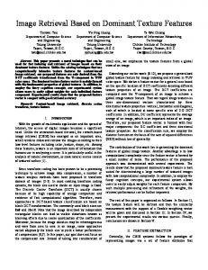
priori the angle θ∗ that gives the best alignment, we have to search over a set of possible rotations by minimizing d(Q, I−θ ) over θ. Notice that when Q and I are in fact two rotated versions of the same image, the angle θ∗ , for which the minimum is achieved in (23), should be close to their exact relative angle, that is, the angle one needs to rotate clockwise the image Q in order to get I . Thus, one way to evaluate the performance of the above rotation-invariant similarity function (23), is to verify whether the estimated angle θ∗ is actually close to the real relative angle between two physically rotated versions of the same image. Besides, this functionality may be also useful on its own for many practical applications to find out approximately this ¯ I−θ ) given by (23), for the Bark relative angle. Fig. 1(b) illustrates this by showing the function d(Q,
texture sample obtained from the Brodatz database. The rotation-invariance property of the similarity function (23) is also illustrated in Fig. 2, where the query image Q (Bark) and the database image I (Water and Leather) belong to different texture ¯ φ , I−θ ) (as a function of θ), that is, classes. Each curve in Fig. 2(a) corresponds to the distance d(Q
the distance between the four versions of the Bark image (original (φ = 0o ) and three rotated versions (30o , 60o , 120o )) and the original Water image rotated clockwise at several angles θ ∈ Θ. Similarly, each
19
curve in Fig. 2(b) corresponds to the distance between the same four versions of the Bark image and the clockwise rotations, at several angles θ ∈ Θ, of the rotated version of Leather image at 90o . It is clear that these curves are approximately shifted versions of each other, which shows (experimentally) the rotation-invariance property of the proposed similarity function (23). However, the expression of this similarity function is quite complicated and norm-dependent and thus, it is difficult to provide an analytical expression for the optimal angle θ∗ , that is, the angle that achieves the minimum in (23). As we can also see in both cases of Fig. 2, the curve corresponding to the version of Bark rotated at φ = 120o has a higher amplitude than the other three curves. This is due to the non-homogeneous nature of the Bark texture image. Besides, both of the higher amplitude curves seem to have a similar peak-to-peak range. However, it is important to note that this higher amplitude does not affect the rotation invariance property since the same phenomenon will appear when comparing the query texture image to the various texture images of the different classes. Notice also how in Fig. 2(a), all the curves corresponding to the Water texture are located vertically at lower positions than the same curves corresponding to the Leather texture (Fig. 2(b)). If we represent the texture information using the signature S instead of SE , the distance between two images Q and I is measured using (23), by taking only the first L summands. Moreover, under a Gaussian assumption (Gaussian signature), (23) can be simplified and takes the following form [24] d¯g (Q, I) = min θ
L X
kClQ − F(−θ)ClI FT (−θ)k ,
(26)
l=1
where, in this case, Cl denotes the matrix with elements being the covariances between pairs of subbands at the l-th pyramid level. It is also important to notice that, in the proposed retrieval method, we achieve rotation invariance through alignment in angle between signatures extracted using a steerable sub-Gaussian model and not by calculating a fixed set of rotation-invariant features valid for all images (which would, for instance, involve diagonalizing matrices and extracting eigenvalues (as in [25] for instance), which has an important complexity) of the same class, namely, the set of images that are rotated versions of each other. C. Computational complexity As mentioned before, one of the goals of this paper is to design a new texture retrieval system that provides the best compromise between complexity and average retrieval performance. In this section, we compare the computational complexity of the retrieval technique proposed in this work, with the
20
−3
7
x 10
Rotation−invariant Frobenius distance
6
Bark.030
5
4
3
2
1
0
0
20
40
Bark.120
60
80
100
120
140
160
180
Angle [in degrees]
(a)
(b)
¯ (a) Bark physically rotated at 30 and 120 degrees, (b) d(Q, I−θ ) for J = 4. Notice that the minimum is achieved for
Fig. 1.
Rotation−invariant Frobenius distance (Eq. 23)
Rotation−invariant Frobenius distance (Eq. 23)
approximately θ∗ = 90 degrees, which is the exact relative angle between the two texture samples.
6 5.5 5 4.5 4 3.5 3 φ=0 φ=30 φ=60 φ=120
2.5 2 1.5
0
20
40
60
80
100
120
Angle [in degrees]
(a)
140
160
180
13
φ=0 φ=30 φ=60 φ=120
12 11 10 9 8 7 6 5
0
20
40
60
80
100
120
140
160
180
Angle [in degrees]
(b)
¯ φ , I−θ ), as a function of θ, between four versions of Bark (original (φ = 0o ) and three physically rotated Fig. 2. Distance d(Q at φ = 30o , 60o , 120o ) and (a) the original image Water, (b) the image Leather rotated at 90o .
21
complexity of three other rotation-invariant texture retrieval methods that have been proposed before and which, to the best of our knowledge, represent the current state-of-the-art: 1) M1 [24]: this method makes a Gaussian assumption for the statistics of the pyramid coefficients and uses a rotation-invariant similarity function based on the Frobenius norm of differences between covariance matrices. 2) M2 [16]: in contrast with M1, this retrieval scheme assumes that the marginal and joint statistics of the pyramid coefficients are best described using members of the family of SαS and multivariate sub-Gaussian distributions. Then, it applies a Gaussianization procedure that consists in extracting the signature of each texture image based on second-order statistics, followed by a rotation-invariant version of the KLD to measure the similarity. 3) M3 [25]: this method is the best current representative within the category of rotation-invariant texture retrieval methods that are based on the statistical fitting of the steerable pyramid coefficients using an HMM. The retrieval method proposed in this paper, as well as the methods M1 and M3, consist of two main components, namely i) the Feature Extraction (FE) and ii) the Similarity Measurement (SM). On the other hand, method M2 has one more additional component, which consists of a Gaussianization procedure applied before the FE step, adding therefore more complexity to the whole retrieval process. In the subsequent analysis, the computational cost is expressed as a function of the number of operations required, where an “operation” is defined as the pair consisting of a multiplication between two numbers and a summation (a · b + c). Let M × M denote the dimension of the original image, which is decomposed via an L-level steerable pyramid with J basic orientations and P to be equal to the neighborhood size that is used during the Gaussianization process in method M2. In addition, let K denote the number of matrices contained in the selected signature, which varies depending on whether we exploit only intra-level, or both intra- and inter-level dependencies, that is, K = L or K = 2L − 1. First, we compare the complexity of the FE step for the four methods, including our proposed retrieval system. Using the above notation, the computational cost of the FE step of our method is approximately equal to K · J 2 · O(M 2 ), where O(M 2 ) is the approximate cost for the computation of the covariation between a pair of subbands using the FLOM covariation estimator of (6). Assuming that the steerable pyramid is constructed without subsampling between consecutive levels, the constant in the O(·) function is small, at the order of 2. Regarding methods M1 and M2, the cost of extracting the signature of an image is of order K · [J(J +
22
1)/2] · O(M 2 ), since both methods estimate covariances between pairs of subbands, which requires
approximately the same order of numerical operations as the estimation of covariations (the constant in the O(·) function is of order 1). In addition, the covariance matrices are symmetric, in contrast to the covariation matrices and thus, in methods M1 and M2, we have to estimate [J(J + 1)/2] elements per matrix, instead of J 2 covariations for each matrix of the signature of the texture retrieval scheme proposed in this work. Taking into consideration that in practice the value of J is usually 3 or 4 and does not depend on the image size, we can conclude that the computational cost of the FE step of our proposed method (K · J 2 · O(M 2 )) is very close to the cost of methods M1 and M2 (K · [J(J + 1)/2] · O(M 2 )). Finally, the cost of the FE step for the HMM-based method M3 is difficult to be estimated with precision, since it employs the Expectation Maximization (EM) algorithm using the ML criterion [20] to estimate the model parameters and thus, it may not even converge in some cases. In order to give a rough estimation of the computational cost of method M3 we argue as follows. The FE step consists of estimating (2L−1) hidden states and (2·L·J) eigenvalues corresponding to the (2L) covariance matrices (each one of dimension J × J ) of the Gaussian densities used in the model. The Expectation step of the EM algorithm is particularly difficult in this case because of the increased interplay between the states. Besides, for an HMM, the complexity of each iteration of EM is linear in the number of observations, that is, the number of subband coefficients in this case. Since method M3 constructs a steerable pyramid by subsampling between adjacent levels, the total number of wavelet coefficients for an L-level pyramid with J orientations per level is equal to JM 2 (1 − 4−L )/3. The total number of model parameters to be estimated is equal to (2L − 1) + 2L J(J+1) , where 2L J(J+1) is the total number of covariances due 2 2 to the symmetry of the 2L covariance matrices. Notice that an additional computational cost is required to perform the eigenvalue decomposition of the covariance matrices in order to obtain their eigenvalues. However, we consider this specific cost to be negligible (as compared to the rest of costs), since in practice the value of J is at most 3 or 4 and thus the dimension of the covariance matrices is very low. Therefore, the computational cost of the FE step of method M3 is of order [(2L − 1) + 2LJ] · O(JM 2 (1 − 4−L )/3), where the constant in the O(·) notation depends on the number of iterations required for the EM algorithm to converge. As a general conclusion, with respect to the computational cost of the FE step of the four methods, the cost of our proposed retrieval technique is approximately equal to the costs of methods M1 and M2, whereas taking into account the usual practical values of L and J , which are usually set to at most 3 or 4, we can conclude that the corresponding cost of method M3 is comparable with the costs of the other three methods only if the EM algorithm converges in very few iterations. For instance, for L = 3 and J = 3
23
the EM algorithm should converge in no more than 5 iterations. Unfortunately, such a fast convergence is not guaranteed a priori, making in practice the FE step of method M3 more computationally expensive, in general, than the FE step of the other three methods. Regarding the SM step, the approach proposed in this work as well as the techniques M1 and M2, all apply Newton’s method to minimize a rotation-invariant similarity function. The computational cost for performing the minimization in these three methods is basically the same, due to the high smoothness of the corresponding expressions inside the min operator in (23), as functions of θ. It is also important to note that, when the steering functions have only odd harmonics (as in our case), they oscillate at some finite speed, which implies an upper bound on the slope of these curves. Thus, it can be readily verified that the number of local minima of the rotation-invariant similarity functions in the texture retrieval method proposed here, as well as in M1 and M2, as a function of θ, can be at most equal to twice the number of independent harmonics (which happens to be equal to the number of basic harmonics). In addition, the distance between any two consecutive local minima is lower bounded making it possible to search for them in a few non-overlapping angular intervals. In particular, the application of Newton’s method in these three retrieval schemes converges very rapidly in practice, namely, in at most 5 iterations in each interval (using the middle of each interval as the initial point). The similarity function proposed in this work, requires for each iteration (during the minimization) about K · (3J 3 + 4J 2 + J) operations. The corresponding cost of each iteration for method M1 is equal to K · (3J 3 + 2J), while method M2 requires about K · (5J 3 + J + D), where D denotes the number of operations for the computation of the determinant of a J ×J matrix (see references [16] and [24] for more details). Using an LU decomposition of a J × J matrix, the determinant is computed in J 3 /3 operations, thus, in practical applications the value of D is small, since the value of J is small, usually J = 3 or 4. Finally, the HMM-based method M3, uses Monte-Carlo simulations to evaluate the integral of the KLD, which, for the experimental setup described in the following section, consists of about 64 iterations [25]. In each iteration, data are randomly generated from the query model as trees of wavelet coefficients, and then its likelihood is computed against a candidate model. Thus, the computational cost of each iteration is proportional to the number of subband coefficients, making the SM step of method M3 much more computationally expensive than the corresponding costs of the other three methods, which depend only on the parameters of the steerable pyramid (L, J ), which are much smaller than the dimension of the images (M × M ). Note that in the above analysis, the computational cost of each method during the SM step, except for method M3, is expressed only as a function of K and J . This is because of the fact that the computational
24
cost for the estimation of the matrices constituting the signature of each method, which depends on M , was taken into account during the analysis for the computational complexity of the FE step, and thus the signature size that determines the computational cost depends only on K and J , since these matrices are already available during the SM. Moreover, it is very important to take also into account that method M2 applies a Gaussianization process, in addition to the FE and SM steps, which adds a significant computational cost that is approximately equal to L · J · [O(P 3 ) + ( 54 M 2 + 2)P 2 + 14 M 2 P + 14 M 2 ], where O(P 3 ) is the number of operations for the inversion of a P × P matrix. After all this analysis, we conclude the following: • The texture retrieval method proposed in this work has a slightly increased complexity than method
M1; however, as we show in the next section of the experimental results, our method results in a better retrieval performance. • The similarity function of our method is less complex than the similarity function designed in
method M2 after the Gaussianization process; on the other hand, the experimental results presented in the following section, show an increased retrieval performance of method M2 compared with the performance of our proposed method, but this difference in performance is much less than the increase of complexity of M2 due to the additional step of Gaussianization. • Finally, as we analyzed above, the computational costs of the FE and SM steps of our method are
in general lower than the corresponding costs of method M3, while achieving a comparable retrieval performance, as our experimental results show in the next section. Thus, the above observations indicate that the texture retrieval method proposed in this work provides the best compromise among all other methods, in the sense of keeping a reduced complexity and offering a competitive retrieval performance. Table I summarizes the computational costs of our proposed method and those of methods M1, M2 and M3. III. E XPERIMENTAL R ESULTS In this section, we evaluate the efficiency of our overall texture retrieval system and compare it with the performance of the three methods M1, M2 and M3, presented in subsection II-C. In order to evaluate the retrieval effectiveness of our method and perform the comparison with the other methods, we apply the same experimental setup as in [16], [25]. In particular, the image database
25
TABLE I C OMPUTATIONAL COMPLEXITY OF THE RETRIEVAL SCHEMES . Method
Gaussianization step
FE step
SM step
PROPOSED
-
KJ 2 O(M 2 )
Cpr K(3J 3 + 4J 2 + J)
M1.
-
K[J(J + 1)/2]O(M 2 )
CM 1 K(3J 3 + 2J)
M2.
LJ[O(P 3 ) + ( 54 M 2 + 2)P 2
K[J(J + 1)/2]O(M 2 )
CM 2 K(5J 3 + J + D)
[(2L − 1) + 2LJ]O(JM 2 (1 − 4−L )/3)
CM 3 O(JM 2 (1 − 4−L )/3)
+ 14 M 2 P + 14 M 2 ] M3. •
-
M1. Gaussian assumption for the statistics of the pyramid coefficients; Frobenius norm-based similarity function of differences between covariance matrices. M2. multivariate sub-Gaussian assumption for the statistics of the pyramid coefficients + Gaussianization; rotation-invariant version of the KLD between multivariate Gaussians as a similarity function. M3. HMM-based statistical fitting of the pyramid coefficients.
•
M × M : the dimension of the original image.
•
L: number of steerable pyramid levels.
•
J: number of basic orientations per level.
•
K: number of matrices contained in the selected signature (K = L or K = 2L − 1).
•
P : neighborhood size that is used during the Gaussianization process.
•
D: number of operations for the computation of the determinant of a J × J matrix.
•
{Cpr , CM 1 , CM 2 } ≈ 5, CM 3 ≈ 64: number of iterations for the minimization of the similarity function. ¡ ¢ g(n) = O f (n) ⇔ ∃ 0 < c1 < c2 and n0 s.t. c1 f (n) ≤ g(n) ≤ c2 f (n) ∀ n ≥ n0
•
consists of 13, 512 × 512 Brodatz texture images obtained from the USC SIPI database11 (cf. Fig. 3). Each of them was physically rotated at 30, 60 and 120 degrees, before being digitized. Then, the texture image dataset was formed by taking 4 non-overlapping 128 × 128 subimages each from the original images at 0, 30, 60 and 120 degrees. Thus, the dataset used in the retrieval experiments contains 208 images that come from 13 texture classes. We implemented a 3-level steerable pyramid decomposition with J = 2 basic orientations, φ1 = 0, φ2 = π/2, which means that the steering functions are [27]:
f1 (θ) = cos(θ) , f2 (θ) = f1
³π 2
´ − θ = sin(θ)
The histogram of the estimated characteristic exponent values for the 208 textures is shown in Fig. 4. 11
http://sipi.usc.edu/services/database
26
Fig. 3. Texture images from the VisTex database, from left to right and top to bottom: 1) Bark, 2) Brick, 3) Bubbles, 4) Grass, 5) Leather, 6) Pigskin, 7) Raffia, 8) Sand, 9) Straw, 10) Water, 11) Weave, 12) Wood, 13) Wool.
We observe that only 28% of the textures exhibit very strong Gaussian statistics, corresponding to α values equal to 2, which belong mainly to pyramid subband coefficients of images 4, 5 and 9. Table II shows the average value of α, over all the pyramid subbands, for each texture class. We observe that images 4, 5 and 9 are exactly those images whose average value of α is closest to 2, compared to the remaining images. In the following, the query is any of the non-overlapping 128×128 subimages in the image dataset. The relevant images for each query are defined as the other 15 subimages from the same original 512 × 512 image. The retrieval performance is evaluated in terms of the percentage of relevant images among the top 15 retrieved images. First, we evaluate the performance of the steerable multivariate sub-Gaussian model combined with the rotation-invariant version of the Frobenius distance, which is proposed in this work. As mentioned before, the signature S , containing the estimated covariation matrices between pairs of subbands at the
27
Relative Frequency
0.25
0.2
0.15
0.1
0.05
0 1
1.1
1.2
1.3
1.4
1.5
1.6
1.7
1.8
1.9
2
Characteristic Exponent
Fig. 4. Histogram of the estimated values for the characteristic exponent, α, for the set of 208 texture images of size 128 × 128.
same decomposition level, is a subset of the enhanced signature SE given by (16). Thus, we extract the signature SE from each texture sample and then, the similarity measurement for the simpler case of using signature S is given from (23) by simply using only the first L matrices of SE . For the 3-level pyramid decomposition that we apply, the signatures S and SE contain 3 and 5 matrices, respectively. Fig. 5 shows the average percentages of correct retrieval rates for each one of the 13 selected texture classes, for the Gaussian signature of size equal to 3, which contains the sample covariance matrices between pairs of subbands at the same level, combined with the corresponding similarity function (26) (method M1) and the sub-Gaussian signatures S and SE , combined with the similarity function (23). We observe that the Gaussian model is better only for 3 classes (4, 5, 9), which are exactly those with the greatest portion of characteristic exponent values (basically) equal to 2. Even for values of α that are slightly smaller than 2, our method provides already a superior performance. Regarding our proposed method, we observe that the enhanced signature SE results in a slightly better retrieval performance than the signature S . Although one could have expected to have a higher increase on the average retrieval rate when using SE instead of S , the reason for this is that for the set of textures that is used, there is not a strong correlation between subbands at adjacent levels, for the selected set of l→(l+1)
textures. This can be verified by examining the off-diagonal elements of the CI
matrices, which
28
TABLE II AVERAGE VALUE OF α, OVER ALL THE PYRAMID SUBBANDS , FOR EACH TEXTURE CLASS .
Texture Class
Aver. α
Texture Class
Aver. α
1
1.8056
8
1.8452
2
1.6512
9
1.9539
3
1.6992
10
1.7563
4
1.9637
11
1.9257
5
1.9695
12
1.7939
6
1.8692
13
1.9266
7
1.8741
have relatively small amplitudes compared with the corresponding elements of the ClI matrices. Due to the increased computational complexity, the enhanced signature should be employed only when a stronger inter-scale correlation is present12 . In order to focus on the non-Gaussian case (the usual case found also in practice in natural images), we omit the 3 “undesired” classes with the strong Gaussian behavior and repeat the above experiment for the remaining set of 10 original, non-rotated textures (thus, giving 160 non-overlapping subimages). Table III shows the corresponding average retrieval rates for the subset of 10 texture classes, for the Gaussian signature of size equal to 3, which contains the sample covariance matrices between pairs of subbands at the same level, combined with the corresponding similarity function (26) (method M1) and the sub-Gaussian signatures S and SE , combined with the similarity function (23). As expected, there is a significant improvement of the average retrieval performance when the pyramid coefficients follow a distinct heavy-tailed non-Gaussian distribution. Fig. 6 shows the average retrieval rates for each individual texture class, of the HMM-based method M3, the method M2 that applies a Gaussianization process on the pyramid coefficients and the method proposed in this work using the enhanced signature SE . It is clear that, for the texture classes whose marginal and joint distributions between the subband coefficients present a heavy-tailed non-Gaussian behavior, our proposed texture retrieval method outperforms the method based on HMMs (which, in 12
To the best of our knowledge, there does not exist electronic databases containing rotated versions of texture images, other
than the one we use here.
29
Gaussian signature sub−Gaussian S sub−Gaussian S
Average Retrieval Rate (%)
E
100 80 60 40 20 0
1
2
3
4
5
6
7
8
9
10
11
12
13
Texture Class
Fig. 5.
Average percentages (%) of correct retrieval rate for each individual texture class. TABLE III
AVERAGE RETRIEVAL RATE (%) IN THE TOP 15 MATCHES , FOR THE SUBSET OF 160 (128 × 128) TEXTURES WITH HEAVY- TAILED MARGINAL DISTRIBUTIONS OF THE PYRAMID SUBBANDS .
Methods Gaussian signature
S
SE
&
&
&
Frobenius (26)
Frobenius (23)
Frobenius (23)
80.18
90.52
92.01
addition, has a larger computational cost in practice), while at the same time maintaining a high retrieval performance, which is comparable to the performance of the method M2, which applies a Gaussianization step before feature extraction. Again, we observe that only for the classes 4,5 and 9, whose marginal distribution of each subband is close to a Gaussian, the rotation-invariant method proposed in this work results in the lowest retrieval performance among the three methods compared in this figure. Even though for the set of texture images that we use in our experiments, the retrieval performance
30
HMM−based (method M3) SG (with Gaussianization) & KLD (method M2) E
sub−Gaussian S
Average Retrieval Rate (%)
E
100 80 60 40 20 0
1
2
3
4
5
6
7
8
9
10
11
12
13
Texture Class
Fig. 6.
Average percentages (%) of correct retrieval rate for each individual texture class.
of the method M2 is slightly better than the performance of the method proposed in this work, as mentioned in subsection II-C, notice also that it has a substantially higher computational complexity due to the Gaussianization procedure. Thus, in the case of a retrieval system with limited computational resources, the implementation of the rotation-invariant scheme proposed here preserves a high retrieval efficiency, while keeping a reasonably low complexity. In conclusion, our method provides an average retrieval performance that is: a) superior to the method M1, while keeping a similar complexity, b) superior to the method M3, while keeping at the same time even a lower complexity, c) competitive (slightly inferior) with the method M2, which has a substantially higher computational complexity. IV. C ONCLUSIONS In this paper, we describe the design of a rotation-invariant texture retrieval system that exploits the nonGaussian heavy-tailed behavior of the distributions of the subband coefficients, representing the texture information via a steerable pyramid. In particular, we construct a steerable multivariate sub-Gaussian model, which relates the fractional lower-order statistics of a rotated image with those of its original version. We perform the similarity measurement between two images by inverting this model, which is
31
equivalent to performing a signature alignment in angle, and minimizing a rotation-invariant similarity function based on the Frobenius matrix norm. The motivation for the development of the proposed rotation-invariant texture retrieval system was the increased computational complexity of our recently introduced method [16], which includes a Gaussianization step before extracting the image signatures, combined with the implementation of a rotationinvariant version of the KLD between multivariate Gaussian densities. We illustrate that, when the marginal and joint distributions of the subband coefficients are heavy-tailed (the usual case encountered in practice with natural images), the proposed steerable sub-Gaussian model achieves a high retrieval performance, while maintaining a sufficiently lower computational complexity. Finally, the experimental results in [16] support our hypothesis about the fact that a statistical similarity function is often more appropriate than a deterministic one. Thus, a future research direction for the improvement of the retrieval performance of the retrieval method proposed in this work, is to study the construction of a rotation-invariant statistical similarity measure, such as the KLD, between multivariate sub-Gaussian distributions, to be used instead of a deterministic norm-based measure. Additional future work could involve extension to non-homogeneous textures by using segmentation. R EFERENCES [1] J. Ashley, M. Flickner, J. Hafner, D. Lee, W. Niblack, and D. Petkovic, “The Query by Image Content (QBIC) system,” in Proceedings of the 1995 ACM SIGMOD Intl. Conf. on Management of data, (New York, U.S.), pp. 475–, ACM Press, 1995. [2] S. Belongie, J. Malik, and J. Puzicha, “Matching shapes,” in Proc. of Intl. Conf. on Computer Vision, Vancouver, Canada, 2001. [3] B. Manjunath, J. R. Ohm, V. Vasudevan, and A. Yamada, “Color and texture descriptors,” IEEE Trans. Circuits and Syst. Video Tech., vol. 11, pp. 703–715, June 2001. [4] J. Malik and P. Perona, “Preattentive texture discrimination with early vision mechanisms,” Journal of Optical Soc. Am., vol. 7(5), pp. 923–932, May 1990. [5] S. Mallat, A Wavelet Tour of Signal Processing. Academic Press, 1998. [6] P. Wu, B. S. Manjunath, S. Newsam, and H. D. Shin, “A texture descriptor for browsing and similarity retrieval,” Signal Processing: Image Communication, vol. 16, pp. 33–43, 2000. [7] M. Unser, “Texture classification and segmentation using wavelet frames,” IEEE Trans. on Image Processing, vol. 4, pp. 1549–1560, Nov. 1995. [8] M. K. Mihcak, I. Kozintsev, K. Ramchandran, and P. Moulin, “Low-complexity image denoising based on statistical modeling of wavelet coefficients,” IEEE Signal Processing Letters, vol. 6(12), pp. 300–303, Dec. 1999. [9] S. G. Mallat, “A theory for multiresolution signal decomposition: the wavelet representation,” IEEE Trans. Pattern Anal. Machine Intell., vol. 11, pp. 674–692, July 1989.
32
[10] E. P. Simoncelli, “Statistical models for images: Compression, restoration and synthesis,” in 31st Asilomar Conf. on Signals, Systems and Computers, (Pacific Grove, CA), pp. 673–678, IEEE Computer Society, 1997. [11] S. G. Chang, B. Yu, and M. Vetterli, “Adaptive wavelet thresholding for image denoising and compression,” IEEE Trans. on Image Processing, vol. 9, pp. 1532–1546, Sep. 2000. [12] M. N. Do and M. Vetterli, “Wavelet-based texture retrieval using generalized Gaussian density and Kullback-Leibler distance,” IEEE Trans. Image Processing, vol. 11, pp. 146–158, Feb. 2002. [13] G. Tzagkarakis and P. Tsakalides, “A statistical approach to texture image retrieval via alpha-stable modeling of wavelet decompositions,” 5th International Workshop on Image Analysis for Multimedia Interactive Services, Lisboa, Portugal, April 21-23 2004. [14] G. Samorodnitsky and M. S. Taqqu, Stable Non-Gaussian Random Processes: Stochastic Models with Infinite Variance. New York: Chapman and Hall, 1994. [15] C. L. Nikias and M. Shao, Signal Processing with Alpha-Stable Distributions and Applications. New York: John Wiley and Sons, 1995. [16] G. Tzagkarakis, B. Beferull-Lozano, and P. Tsakalides, “Rotation-Invariant Texture Retrieval with Gaussianized Steerable Pyramids,” IEEE Trans. Image Processing, vol. 15(9), pp. 2702–2718, Sep. 2006. [17] J. Huang, “Study on the correlation properties of wavelet transform coefficients and the applications in a neural networkbased hybrid image coding system,” CISST’03, Las Vegas, USA, June 22-26 2003. [18] J. Portilla and E. P. Simoncelli, “A parametric texture model based on joint statistics of complex wavelet coefficients,” International Journal of Computer Vision, vol. 40, pp. 49–71, Dec. 2000. [19] G. Cross and A. Jain, “Markov random field texture models,” IEEE Trans. Patt. Anal. Mach. Intell., vol. 5, no. 1, pp. 25–39, 1983. [20] M. S. Crouse, R. D. Nowak, and R. G. Baraniuk, “Wavelet-based statistical signal processing using hidden markov models,” IEEE Trans. on Signal Processing (Special issue on Wavelets and Filterbanks), pp. 886–902, April 1998. [21] H. Greenspan, S. Belongie, R. Goodman, and P. Perona, “Rotation invariant texture recognition using a steerable pyramid,” in Proc. Int. Conf. on Pattern Recognition, Jerusalem, Israel, vol. 2, pp. 162–167, 1994. [22] G. M. Haley and B. S. Manjunath, “Rotation invariant texture classification using modified Gabor filters,” in Proc. IEEE Int. Conf. Image Processing, Washington, DC, vol. 1, pp. 262–265, Nov. 1995. [23] G. M. Haley and B. S. Manjunath, “Rotation-invariant texture classification using a complete space-frequency model,” IEEE Trans. Image Processing, vol. 8, pp. 255–269, Feb. 1999. [24] B. Beferull-Lozano, H. Xie, and A. Ortega, “Rotation-invariant features based on steerable transforms with an application to distributed image classification,” in Proc. of IEEE Intl. Conf. on Image Processing, Barcelona, Spain, Sep. 2003. [25] M. N. Do and M. Vetterli, “Rotation invariant texture characterization and retrieval using steerable wavelet domain hidden Markov models,” IEEE Trans. on Multimedia, vol. 4, pp. 517–527, Dec. 2002. [26] F. Liu and R. W. Picard, “Periodicity, directionality, and randomness: Wold features for image modeling and retrieval,” IEEE Trans. Patt. Anal. Mach. Intell., vol. 18, pp. 722–733, July 1996. [27] W. T. Freeman and E. H. Adelson, “The design and use of steerable filters,” IEEE Trans. Patt. Anal. Mach. Intell., vol. 13, no. 9, pp. 891–906, 1991. [28] E. P. Simoncelli, W. T. Freeman, E. H. Adelson, and D. J. Heeger, “Shiftable multi-scale transforms,” IEEE Trans. Information Theory (Special issue on Wavelets), vol. 38(2), pp. 587–607, Mar. 1992.
33
[29] J. P. Nolan, “Parameterizations and modes of stable distributions,” Statistics & Probability Letters, no. 38, pp. 187–195, 1998. [30] J. P. Nolan, “Numerical calculation of stable densities and distribution functions,” Commun. Statist.-Stochastic Models, vol. 13, pp. 759–774, 1997. [31] M. Shao and C. L. Nikias, “Signal processing with fractional lower order moments: Stable processes and their applications,” Proc. IEEE, vol. 81, pp. 986–1010, 1993.
34
L IST OF TABLES I
Computational complexity of the retrieval schemes. . . . . . . . . . . . . . . . . . . . . . . . 25
II
Average value of α, over all the pyramid subbands, for each texture class. . . . . . . . . . . 28
III
Average retrieval rate (%) in the top 15 matches, for the subset of 160 (128 × 128) textures with heavy-tailed marginal distributions of the pyramid subbands. . . . . . . . . . . . . . . . 29 L IST OF F IGURES
1
¯ I−θ ) for J = 4. Notice that the (a) Bark physically rotated at 30 and 120 degrees, (b) d(Q,
minimum is achieved for approximately θ∗ = 90 degrees, which is the exact relative angle between the two texture samples. . . . . . . . . . . . . . . . . . . . . . . . . . . . . . . . . . 20 2
¯ φ , I−θ ), as a function of θ, between four versions of Bark (original (φ = 0o ) Distance d(Q
and three physically rotated at φ = 30o , 60o , 120o ) and (a) the original image Water, (b) the image Leather rotated at 90o . . . . . . . . . . . . . . . . . . . . . . . . . . . . . . . . . . . . 20 3
Texture images from the VisTex database, from left to right and top to bottom: 1) Bark, 2) Brick, 3) Bubbles, 4) Grass, 5) Leather, 6) Pigskin, 7) Raffia, 8) Sand, 9) Straw, 10) Water, 11) Weave, 12) Wood, 13) Wool. . . . . . . . . . . . . . . . . . . . . . . . . . . . . . . . . . 26
4
Histogram of the estimated values for the characteristic exponent, α, for the set of 208 texture images of size 128 × 128. . . . . . . . . . . . . . . . . . . . . . . . . . . . . . . . . 27
5
Average percentages (%) of correct retrieval rate for each individual texture class. . . . . . . 29
6
Average percentages (%) of correct retrieval rate for each individual texture class. . . . . . . 30