Friedrich}@uni-klu.ac.at images of parts of this area [13]. We will refer to the locations where these pictures have to be taken as picture points. In our application.
Routing for Continuous Monitoring by Multiple Micro UAVs in Disaster Scenarios Vera Mersheeva and Gerhard Friedrich1 Abstract. In disaster situation a quickly obtained and regularly updated overview image of an area provides essential information for the rescue mission planning. Such an overview image can be composed from the individual pictures taken by a fleet of Unmanned Aerial Vehicles (UAVs). However, currently drones are remotely controlled by humans during such missions. To the best of our knowledge, no research has been conducted on the problem of UAV routing for such task. Therefore, we propose a method based on the wellknown metaheuristic Variable Neighborhood Search. In particular, we developed two new heuristics to construct the initial solution and an additional neighborhood operator. Computational experiments indicate that solutions obtained by our metaheuristic do not exceed the optimum by more than 26.9% on small scenarios. For the large instances with hundreds of points (where no optimal solution is known) the proposed method constructs feasible solutions in less than one second.
1
INTRODUCTION
Unmanned aerial vehicles (UAVs) are gaining popularity in various areas such as disaster management [13], agricultural surveillance [7], urban terrain surveillance [4], military operations [14], construction site monitoring, etc. In particular, the employment of micro UAVs, i.e. drones that can be carried by a human, achieved high attention in research and applications because of their simple handling and low costs. The goal of our project is to develop a system employing a team of micro UAVs for aerial sensing in disaster situations. A fast first overview image of a target area is very useful for first responders who need to know the current situation. In order to track possible changes of the situation, an overview image should be regularly updated during the whole rescue operation. In this paper we consider the problem of UAVs routing for obtaining these overview images. The use of micro UAVs in a rescue scenario has several restrictions that have to be taken into account. The energy storage (e.g. a battery) of the UAVs has limited capacity (approximately 10 – 45 minutes flight time depending on environmental conditions). Additionally, there may be a single or multiple base stations with loaded spare batteries where the UAVs depart from, return to and can change their energy storage. Due to legal restrictions, drones cannot fly above a certain altitude. Finally, micro UAVs have a limited payload. Due to the reasons mentioned above, drones cannot fly high enough or use sophisticated cameras with wide-angle lenses to take an overview picture of the whole area with one shot. Therefore, an overview image of an area is generated by stitching a set of individual 1
Alpen-Adria-Universit¨at Klagenfurt, Austria, email: {Vera.Mersheeva, Gerhard.Friedrich}@uni-klu.ac.at
images of parts of this area [13]. We will refer to the locations where these pictures have to be taken as picture points. In our application scenarios we have to deal with several hundred such points. Despite the fact that during the last decade many research projects were dedicated to UAV route planning, to the best of our knowledge, all of the related problems differ significantly from the described specification. One related problem, Multi-Depot Multiple UAV Routing Problem [12], does not consider multiple trips by a single vehicle. Problems such as Patrolling Task [9] and Multi-Depot Multi-trip Vehicle Routing Problem [3] do not take into account limitation on battery capacity. In addition, mentioned UAV and Vehicle Routing Problems require exactly one visit at every target point. Since none of the related problems consider all the requirements we have, the existing algorithms cannot be directly applied here. Due to the problem complexity, complete methods (methods that always find the optimal solution) exploited by mixed-integer programming, constraint-based programming or logic programming are not applicable for the real-life scenarios that contain several hundred picture points. To underline this assertion we provide run times for employing constraint-based programming to our problem specification. As a consequence, only a heuristic approach, that does not guarantee the optimum but is sufficiently efficient, should be used for this new type of problem. In this paper we propose two different construction heuristics to obtain an initial feasible solution and a metaheuristic approach to improve the initial solution iteratively. The construction heuristics exploit the basic ideas of the Solomon’s insertion heuristic [15] and Clarke and Wright savings algorithm [2]. The metaheuristic is based on the well-known Variable Neighborhood Search (VNS) introduced by Mladenovic et al. [10] which was successfully applied to a number of vehicle routing problems, e.g. the Periodic Vehicle Routing Problem [6]. Computational results show that a solution obtained within ten seconds by our method is at most 26.9% far away from the optimum. Additionally, feasible solutions were obtained in less than one second for the problem instances with over 400 points. This paper is organized as follows. A problem description is given in Section 2. Sections 3–6 contain detailed explanations of the developed algorithms. Section 7 presents computational results. Finally, in Section 8 we summarize the achievements and provide ideas for the future research.
2
PROBLEM SPECIFICATION
Given a set of waypoints W partitioned in a set of picture points P = {p1 , ..., pm } and a set of base stations B and a matrix D of distances between waypoints. This matrix is symmetric, i.e. di j = d ji . Additionally, between all triples of waypoints the triangular inequal-
ity has to be satisfied, i.e. for any three waypoints i, j, k it holds that di j + d jk ≥ dik . A set of energy storage units E (also known as batteries) and a fleet of UAVs V = [v1 , ..., vn ] of possibly different types T are initially located at various base stations. Every drone of a particular type has a certain speed and a limited maximum time of flight with one battery. Both of these parameters can be different for different types of UAVs. Additionally, time intervals needed to take one picture tT P and to change battery tChB are known. Finally, time of the whole mission is restricted to a given value mT . A solution is a set of routes R = {r1 , ..., rn } for all available UAVs. A route ri is a sequence of waypoints [wi,1 , ..., wi,lasti ], for all available UAVs. A solution is feasible if it satisfies the following constraints: 1. A drone v should start and finish its route at the base station bv where it was initially placed, i.e. wv,1 = wv,lastv = bv . 2. A drone v may change its battery only at its initial base station bv . As consequence, its route can contain only picture points or an initial base station, i.e. wv,1 , ..., wv,lastv ∈ P ∪ bv . 3. A vehicle cannot fly with one battery longer than its maximum flight time tmax . 4. The time of the whole mission should not exceed the limit mT . 5. Every picture point is visited at least once. 6. At every base station the number of battery changes should not exceed the number of spare batteries of the correspondent type. 7. The number of routes is equal to the number of drones. As it was mentioned in the introduction, our problem consists of two tasks. The first task is to obtain the first overview image of an area as quickly as possible. The second task is regularly repeated visits of picture points which we call continuous monitoring. Therefore, the objective is split in two parts with different priorities: Top priority Within the first coverage, the objective is to minimize the last arrival time at picture point. Second priority For the continuous monitoring, a goal function aims at maximizing number of visits and making the frequency of these visits at all picture points more equal. It is calculated as follows: 2 → min, ∑ ∑ ∆tvisit p∈P visit∈Visits p
where Visits p is a set of all visits at picture point p; ∆tvisit is a time interval from the current visit till the next visit (or till the mission time mT in case of the last visit).
3
VARIABLE NEIGHBORHOOD SEARCH
As any metaheuristic, VNS starts with an initial solution obtained by using a construction heuristic and iteratively improves the found solution. A a set of operators Nk (k = 1, . . . , kmax ) can be applied to the current state (current solution) resulting in a set of successor states. The set of successor states generated by applying an operator Ni is called a neighborhood. From such a neighborhood a state is randomly selected and improved by local search techniques. If no improvement can be found, the neighborhood is switched to the next one, i.e. another operator is applied. An acceptance phase evaluates whether the current solution is accepted or not. In short, the basic VNS steps are as follows: 1. Obtain an initial solution xi by exploiting a heuristic which can generate a feasible solution. Select a set of operators with cardinality kmax which will be applied to modify a solution. Choose a
stopping condition (e.g. a limit on computational time or on the number of iterations). 2. Set current solution x ← xi . Repeat the following steps until the stopping condition is met: (a) Set index of operator k ← 1; (b) Repeat the steps below until k = kmax : i. Shaking. Generate a new solution x0 by applying kth operator to a current solution; ii. Local search. Apply some local search method to x0 which outputs x00 as a local optimum; iii. Acceptance phase. If the local optimum x00 is better than solution x or some acceptance criterion is met, set x ← x00 and continue to search starting with the first operator (k ← 1); otherwise, set k ← k + 1. In the following subsections these steps will be described in more detail for the tasks of obtaining the first coverage and performing continuous monitoring.
4 4.1
INITIAL SOLUTION Task of Obtaining the First Coverage
To obtain a set of routes for the first coverage we used slightly modified standard approaches such as the parallel Clarke and Wright savings algorithm [2] and clustering in combination with the Christofides algorithm [1]. For clustering a hybrid method was created based on the k-means [8] and the k-medoids clustering [11] algorithms. In this method, the centre of a cluster is the picture point the closest to the Euclidian centre. The obtained solution is an input for the planning problem of continuous monitoring.
4.2
Task of Continuous Monitoring
Whereas for the previous task we can use existing approaches, to the best of our knowledge, no method exists for the problem of continuous monitoring. However, successful heuristics introduced for related problems are first-choice candidates for the adaptation to this task. In particular, we focused on two different approaches; the Clarke and Wright saving strategy and the Solomon’s insertion heuristic. Their adaptations are presented in this section and evaluated in Section 7. Modified Clarke and Wright savings algorithm (CW) This savings algorithm was originally developed for the Travelling Salesman Problem (TSP) [2]. It starts from the infeasible solution that consists of routes of type b − pi − b for all target points (picture points) pi , i ∈ [1, m], and a single given depot (base station) b, B = {b}. Then all possible pairs of points pi and p j (i, j ∈ [1, m]; i 6= j) are sorted in descending order by the savings value s(pi , p j ) calculated as: s(pi , p j ) = d pi b + dbp j − d pi p j . Connections are established iteratively between points with highest saving values, where such a connection does not violate the TSP constraints. Since the problem of continuous monitoring differs significantly from the TSP, the savings algorithm was modified to deal with the extensions shown in Table 1. The resulting CW Algorithm is described in Algorithm 1. Two routes ri and r j are joined by connecting the “savings” points pi and p j. Therefore, two last conditions in the line 12 in Algorithm 1 define that for the successful connection these points should be at the beginning or in the end of these routes.
Table 1.
Modifications applied to the original savings algorithm
Extensions Multiple base stations Multiple vehicles with possibly multiple trips Several visits at every picture point
Modifications Savings values are calculated for every pair of picture points and a base station closest to these points. During the computational process a drone is assigned to a route. Routes with two assigned UAVs from different base stations cannot be connected. The modified algorithm is applied to the same set of picture points, as long as there are spare batteries.
The function connect(ri,rj) returns true if two routes ri and r j were successfully connected into route ri ∪ r j and return false otherwise. They are connected if they do not start at different base stations and the resulting route will not violate battery capacity limitation. The function assignUAV(ri ∪ r j) assigns a UAV and its initial base station to the route ri ∪ r j. If any UAV v ∈ V was assigned with either ri or r j then select v. If both ri and r j had no assigned vehicle then such drone is chosen which has a spare battery, can start following the route ri ∪ r j earlier than others and is close. On choosing a UAV the available batteries E are decremented. Finally, function join(R, Rc ) inserts points from routes rc ∈ Rc to routes r ∈ R of the correspondent UAVs. Algorithm 1: Modified savings algorithm input : problem specification and a set of routes R1 = {r11 , ..., r1n } for the first coverage, where n is a number of vehicles output: a set of routes R for both tasks: first coverage and continuous monitoring 1 2 3
4 5 6 7 8
9 10 11 12
13 14 15 16 17 18 19
set R ← R1 ; set a list of savings S ← {}; for pi , p j ∈ P(pi 6= p j do calculate s(pi , p j , b), where � � b = arg minbi ∈B dbi pi + d p j bi ; set S ← S ∪ s(pi , p j , b); end sort S in descending order; repeat assign a set of routes for current coverage Rc ← [[pi ] |pi ∈ P];
points one after another at more profitable positions in the best routes chosen by an evaluation value. Since our problem deviates in several aspects from [15], such as no time windows but multiple coverage, a new insertion heuristic has to define a more suitable evaluation value and an order in which picture points will be inserted. A good solution for the continuous monitoring problem is a solution where frequencies of visits at points are close to equal. Consequently, our algorithm should eliminate a situation where some points have significantly more visits than others and first insert those points which were visited long time ago. Therefore, all picture points are ordered in a queue Q = {q1 , ..., qm } in ascending order by their first arrival time. In every insertion iteration we take the first point of the queue Q. Our new evaluation value must choose a route (1) which ends with a picture point located as close as possible to the insertion point q1 and (2) whose vehicle can arrive at the insertion point earlier. The first parameter aims at optimizing the distance travelled by every vehicle whereas the second parameter tries to shorten the time between visits� at the insertion point. Thus, this evaluation value for the route r = w1 , ..., wlastr is calculated as follows: f (q1 , r) = α1 · dwlastr ,q1 · scale + α2 · twlastr ,q1 . Variable twlastr ,q1 is a possible arrival time to a point q1 if it is inserted in the route r. The scale coefficient is set to a value so that the orders of magnitude of arrival time and distance between points are the same. The weights α1 and α2 = 1 − α1 reflect how much every parameter (distance and arrival time) influences the final decision. Value α1 = 0.7 showed the best results for our problem. All steps of the queue-based insertion heuristic are shown in Algorithm 2. Eb,r refers to batteries suitable for the vehicle associated to route r and located at base station b. Algorithm 2: Queue-based insertion heuristic input : problem specification and a set of routes R1 = {r11 , ..., r1n } for the first coverage, where n is a number of vehicles output: a set of routes R for both tasks: first coverage and continuous monitoring 1 2
3 4
for s(pi , p j , b) ∈ S do set ri ← r ∈ Rc , where pi ∈ r; set r j ← r ∈ Rc , where p j ∈ r; if (ri 6= r j) and (wri,1 = pi or wri,lastri = pi ) and (wr j,1 = p j or wr j,lastr j = p j ) then if connect(ri,rj) then assignUAV(ri ∪ r j); end end end join(R, Rc ); until E = 0; /
Queue-based insertion heuristic (QI) This heuristic is based on Solomon’s insertion heuristic [15] which was first introduced for the Vehicle Routing Problem with Time Windows. The algorithm inserts
5 6 7 8 9 10 11 12 13 14 15
5
set R ← R1 ; set a queue Q ← [q1 , ..., qm ] s.t. tqi ≤ tqi+1 , qi , qi+1 ∈ P, i ∈ [1, m − 1]; repeat set a chosen route r ← arg minri∈R f (q1 , ri); if f (q1 , r) = ∞ then set Q ← Q \ {q1 }; else if r ∪ {q1 } does not violate energy constraint then set r ← r ∪ q1 ; else set r ← r ∪ b ∪ q1 , where b ∈ B; Eb,r 6= 0; / end set Q ← {q2 , ..., qm , q1 }; end until Q = 0; /
SHAKING PHASE AND LOCAL SEARCH
The purpose of the shaking step (see Section 3, Step 2(b)i) is to modify the current solution with retaining those parts contained in an
optimal solution in order to give way for improvements and escape from the local optimum. After the shaking step, changed routes are optimized by local search (see Section 3, Step 2(b)ii). In the following we describe these steps for the first coverage and continuous monitoring.
5.1
Table 2. Neighborhood operators for the first coverage and continuous monitoring problems First coverage Continuous monitoring k Operator Max. segment k Operator Max. segment length length 1 cross min(1, n) 1 move min(1, n) 2 cross min(2, n) 2 move min(2, n) 3 cross min(3, n) 3 move min(3, n) 4 cross min(4, n) 4 cross min(1, n) 5 cross min(5, n) 5 cross min(2, n) 6 cross min(6, n) 6 cross min(3, n) 7 move min(1, n) 7 cross min(4, n) 8 move min(2, n) 8 cross min(5, n) 9 move min(3, n) 9 cross min(6, n)
Task of Obtaining the First Coverage
Cross-exchange and move operators are the most widely used interroute operators [6]. The cross-exchange operator exchanges two equally long segments of two routes. For instance, in Figure 1 segments {x1 , ..., y1 } and {x2 , ..., y2 } are removed from their routes r1 , r2 and are inserted in the other routes r2 , r1 . The move operator relocates a segment of one route to another. Segment {x1 , ..., y1 } is removed from its current route and is added to another route as shown in Figure 2. Both operators choose routes, segments and their length randomly. The segment length can take any values up to the maximum segment length shown in Table 2 for every applied operator. Variable n is the shortest length of the two chosen routes; k is the sequential number of an operator (see Section 3).
Figure 1. A cross-exchange operator for routes r1 (black) and r2 (grey)
10 11 12
insert insert insert
Max. number of points min(1, n) min(2, n) min(3, n)
introduce an insert operator which inserts points at random positions into a randomly chosen route. Table 2 shows the maximum possible number of insertion points for this operator. The chosen order was determined by our experiments described in Section 7. As in the previous task, 2-opt and 3-opt are used as local search strategies. Their changes are accepted if the flight time of a route decreases since this allows additional revisits of picture points and reduces the goal function of continuous monitoring.
6
ACCEPTANCE PHASE
The purpose of the acceptance phase is to determine whether the current solution should be chosen. Various strategies can be exploited (e.g. simulated annealing) where a non-improved solution is accepted with a certain probability, which decreases over time. Simulated annealing did not give reasonable improvements for our real-life scenarios. Therefore, we use a strategy where only improved solutions are accepted.
7 Figure 2. A move operator for routes r1 (black) and r2 (grey)
For the local search phase we apply the commonly used 2-opt and 3-opt strategies that are special cases of the general k-opt [5] algorithm. This algorithm reconnects every combination of k arcs in the route in all possible ways so that the result is a solution to a TSP. If a new route has a better cost value it is accepted. This procedure is applied as long as no more improvements can be achieved. The obtained solution is called k-optimal. The computational time increases exponentially as the value of k increments. However, benefits from using larger values of k usually do not increase significantly. Therefore, it is common practice to apply only 2-opt and 3-opt.
5.2
Task of Continuous Monitoring
Monitoring is more efficient if picture points are visited more often. Therefore, in addition to the cross-exchange and move operators we
COMPUTATIONAL RESULTS
In order to find routes for the first coverage of an area, existing algorithms were used. Therefore, this task is not considered in this section. Conversely, methods developed for the problem of continuous monitoring should be evaluated in a number of aspects. First of all, the deviation from the optimum is estimated, since the presented methods are not complete and do not necessarily find optimal solution. However, due to complexity this estimation cannot be performed on real-world scenarios. Therefore, the proposed QI and CW heuristics are compared with each other on the large scenarios. Finally, additional tests are conducted on estimation of the best neighborhood structure. We ran all the tests on an Intel Core i7 2.67 GHz system with 4GB RAM. Results of all mentioned tests will be presented below. Comparison of the VNS, QI and CW heuristics with optimum on small-scale scenarios For this test we generated 9 benchmarks with 6 picture points and 2 base stations. Locations of points were chosen randomly so that the first coverage is feasible. Every base station stores 1 drone and 2 – 4 batteries. Mission time is limited by the longest possible mission of a drone. In addition, routes from the first
coverage obtained by the standard Clarke and Wright algorithm are given for all cases since we compare methods for continuous monitoring. In order to compute the optimum, we developed a model employing the constraint modelling language MiniZinc and solved the problem instances with the constraint-based programming solver Gecode. Figure 3 presents the performance of the VNS with and without the improvement phase where initial solutions were found with either the QI or CW heuristics. The improvement phase was stopped after 104 iterations (less than 1 millisecond) for every benchmark. In contrast, finding the optimal solutions took 4832.72 seconds on the average.
Figure 4. An example of the real-world scenario
Figure 3. Deviation from the optimum of QI and CW heuristics and their combinations with VNS
According to the results, solutions returned by QI and CW do not exceed the optimum by more than 26.9% and 50.3% respectively. Moreover, the solutions obtained by a combination of our VNS modification and QI or CW are at most 26.9% and 39.07% off from the optimum. It is important to mention, that the QI heuristic outperformed CW on most instances. Evaluation of QI and CW heuristics on real-life scenarios A set of 36 benchmarks representing real areas of interest were used for this evaluation. Every benchmark contains 46 – 442 picture points and 3 or 6 base stations. Since the whole area has to be covered evenly, picture points are equally distributed over the area excluding obstacle areas. Additionally, a fleet of 3, 6 or 9 UAVs and a set of 3 – 22 batteries are equally distributed between the base stations. Parameters such as drone’s velocity and maximum flight duration are set to the real values of the drones used in the project. Figure 4 shows an instance with the name “442p 1” from our test set . It represents an area around our university and neighbouring buildings and contains 442 picture points marked with small circles and 3 base stations displayed as large filled circles. Areas with no picture points are no-fly zones due to the presence of the obstacles. Figure 5 shows the results obtained by both CW and QI algorithms. According to these results, on most of the smaller scenarios (less than 251 picture points) QI heuristic achieved better results than CW regardless of the number of vehicles, batteries or base stations used. However, CW algorithm outperformed QI on larger instances. QI and CW heuristics found the feasible solutions for all the instances in 355 and 1323 milliseconds respectively. Due to the short computational time, these heuristics are applicable in our domain which requires a fast response. In conclusion, we suggest to use QI for the problems with relatively small number of picture points (≤ 251) and CW for all the other instances.
Evaluation of the neighborhood structure Every neighbourhood operator influences the solution differently and, as consequence, a correct order of the operators is significant for achieving improvements. Therefore, we evaluated various combinations of crossexchange (c), move (m) and insert (i) operators and estimated contribution of the best combination to the final solution. In particular, we considered four possible orders: m-c-i, c-m-i, i-m-c and c-i-m. Table 3 contains the number of times when a particular operator led to a better solution, the average percentage of improvement and the final percentage of improvement for 104 iterations. Sequence mc-i achieved the best average and final improvement values. Since the move and cross-exchange operators make routes shorter, there is more space for inserting new points than in any other combination. Consequently, this sequence decreases goal function the most due to a larger number of visited picture points. These results prove that sequence m-c-i is reasonable and the new insert operator is efficient.
Table 3. Evaluation of different sequencies of neighborhood operators k 1 2 3 4 5 6 7 8 9 10 11 12 Average percentage of improvement Final percentage of improvement
m-c-i m4 m5 m3 c 3 c 4 c 3 c 3 c 2 c 2 i 69 i 9 i 2 0.00121
c-m-i c 3 c 1 c 2 c 2 c 2 c 2 m3 m4 m4 i 56 i 5 i 3 0.00111
i-m-c i 50 i 5 i 4 m3 m2 m0 c 1 c 1 c 0 c 2 c 1 c 2 0.00114
c-i-m c 3 c 4 c 1 c 3 c 2 c 4 i 52 i 8 i 2 m4 m2 m3 0.000999
12.11268 11.13094 11.41604 9.989225
Figure 5. Comparison of QI and CW heuristics on real-life scenarios
8
CONCLUSIONS
In this paper, we proposed a new method based on the standard metaheuristic Variable Neighborhood Search. We developed a new neighborhood operator, i.e. the insert operator, and two new construction heuristics, i.e. the modified Clarke and Wright algorithm (CW) and the queue-based insertion heuristic (QI). The heuristics CW and QI were compared with each other on 36 real-life problem instances which were solved in less than 2 seconds by each algorithm. The CW algorithm outperformed QI on large instances (with more than 251 picture points) whereas QI provided better solutions for small-scale problems. Since our method is not an exact method, it was evaluated regarding its deviation from the optimum where the computation of the optimum was feasible. For these test cases our metaheuristic obtained solutions at most 26.9% worse than the optimum. Finally, several neighborhood structures with a new insert operator were analyzed for choosing the best order. An order with the best final improvements (12.11% on large scenarios) was selected. Additionally, results indicate that the insert operator is efficient since it improved the goal function value significant number of times. In summary, the developed metaheuristic is fast, efficient and scalable for large scenarios. Further research will be conducted on enhancing the proposed method to solve extensions of the specified problem such as no-drone base stations and dynamically changing environments.
ACKNOWLEDGEMENTS This work was supported by Lakeside Labs GmbH, Klagenfurt, Austria and funding from the European Regional Development Fund and the Carinthian Economic Promotion Fund (KWF) under grant KWF20214/17095/24772.
REFERENCES [1] N. Christofides, ‘Worst-case analysis of a new heuristic for the traveling salesman problem’, Technical report, Carnegie-Mellon University, Pittsburgh, USA, (February 1976). [2] G. Clarke and J. W. Wright, ‘Scheduling of vehicles from a central depot to a number of delivery points’, Operations Research, 12, 568– 581, (July/August 1964). [3] B. Golden, S. Raghavan, and E. Wasil, The vehicle routing problem: latest advances and new challenges, Operations Research/Computer Science Interfaces, Springer, 2008. [4] D. Gross, S. Rasmussen, P. Chandler, and G. Feitshans, ‘Cooperative operations in urban terrain (COUNTER)’, in Society of Photo-Optical Instrumentation Engineers Conference, volume 6249, (2006).
[5] K. Helsgaun, ‘An effective implementation of the Lin-Kernighan traveling salesman heuristic’, European Journal of Operational Research, 126, 106–130, (2000). [6] V. C. Hemmelmayr, K. F. Doerner, and R. F. Hartl, ‘A variable neighborhood search heuristic for periodic routing problems’, European Journal of Operational Research, 195, 791–802, (2009). [7] M. Israel, ‘A UAV-based roe deer fawn detection system’, International Archives of Photogrammetry and Remote Sensing, XXXVIII-1/C22, (2011). [8] A. K. Jain, M. N. Murty, and P. J. Flynn, ‘Data clustering: a review’, ACM Computing Surveys, 31, 264–323, (1999). [9] A. Machado, G. Ramalho, J.-D. Zucker, and A. Drogoul, ‘Multi-agent patrolling: An empirical analysis of alternative architectures’, in MultiAgent-Based Simulation, Third International Workshop, pp. 155–170, (2002). [10] Nenad Mladenovic and Pierre Hansen, ‘Variable neighborhood search’, Computers & Operations Research, 24, 1097–1100, (1997). [11] R. T. Ng and J. Han, ‘Efficient and effective clustering methods for spatial data mining’, in Very Large Data Bases, pp. 144–155, (1994). [12] P. Oberlin, S. Rathinam, and S. Darbha, ‘Today’s traveling salesman problem’, Robotics Automation Magazine, IEEE, 17, 70 –77, (2010). [13] M. Quaritsch, K. Kruggl, D. Wischounig-Strucl, S. Bhattacharya, M. Shah, and B. Rinner, ‘Networked uavs as aerial sensor network for disaster management applications’, e & i Elektrotechnik und Informationstechnik, 127, 56–63, (2010). 10.1007/s00502-010-0717-2. [14] C. Schumacher, P.R. Chandler, M. Pachter, and L.S. Pachter, ‘Optimization of air vehicles operations using mixed-integer linear programming’, Journal of the Operational Research Society, 58, 516–527, (2007). [15] M. M. Solomon, ‘Algorithms for the vehicle routing and scheduling problems with time window constraints’, Operations Research, 35, 254–265, (April 1987).