routing in high-speed networks - CiteSeerX

ROUTING IN HIGH-SPEED NETWORKS

A Dissertation Presented by

Ren-Hung Hwang

Submitted to the Graduate School of the University of Massachusetts in partial ful llment of the requirements for the degree of

Doctor of Philosophy May 1993 Department of Computer Science

c Copyright by Ren-Hung Hwang 1993 All Rights Reserved

ROUTING IN HIGH-SPEED NETWORKS

A Dissertation Presented by

Ren-Hung Hwang

Approved as to style and content by: James F. Kurose, Chair Don Towsley, Member Jack C. Wileden, Member Christos G. Cassandras, Member W. Richards Adrion, Department Head Department of Computer Science

Dedicated to My wife, Pey-Lin Su and My parents, Yu-In Yang and Tsung-Hsiung Hwang

ACKNOWLEDGMENTS First and foremost, I wish to thank my advisor, Prof. Jim Kurose. He taught me not just how to get a Ph.D. but how to be a Ph.D. His excellent writing and pedagogic skills and tireless enthusiasm have helped me not only be able to nish this dissertation but also prepare myself as an independent researcher and a great teacher. I especially thank him for his great patience in teaching me how to write a good paper. Without him, a Ph.D. would be just a title to me. It is also a great honor and pleasure to acknowledge Professor Don Towsley, my other advisor, for his technical support, helpful suggestions and insights. His excellent talent in modeling skills has prevented me from being sloppy in formulating my analytical models. Special thanks are due to Prof. Jack Wileden and Prof. George Avrunin. I had the great pleasure of working with them during the second year of my graduate study. I also thank Jack for serving as a thesis committee member and writing recommendation letters on my behalf. My thanks also go to Prof. Christos Cassandras, my other thesis committee member, for his advice and feedback, which were invaluable to my thesis. Thanks are due to many individuals who have helped me in many ways. I am grateful to David Yates for his friendship and his generous willingness to serve as the rst reader of my papers, proposals, and this dissertation. Special thanks are due to Dr. and Mrs. Barrie Yates, David's parents, for providing me very comfortable accommodations in their splendid house when I was working at GTE Laboratories. I also thank Renu Chipalkatti, Dr. Adrian Conway, Dr. Dragomir Dimitrijevtic for giving me an opportunity to work at GTE Laboratories. Special thanks are also due to Dr. Yow-Jong Liu at GTE Laboratories for his warm friendship. I am also grateful to all members, old and new, of the Amherst Chinese Christian Church. I thank them for being my brothers and sisters in Christ. iv

Finally, I must mention the tremendous support I have received from my family. I wish to thank my wonderful Push-Husband-Through (Ph.T.) wife, Pey-Lin Su, for her endless love during my years struggling through graduate school. I also thank my parents who sacri ced themselves to support me nancially and spiritually. Without their eorts, this dissertation would not exist.

v

ABSTRACT ROUTING IN HIGH-SPEED NETWORKS

May 1993 Ren-Hung Hwang B.S., National Taiwan University M.S., University of Massachusetts Ph.D., University of Massachusetts Directed by: Professor James F. Kurose In the 1990s, signi cant advances in ber optic and switching technology have precipitated the current explosion in the amount of research in future high-speed networks. The challenges facing high-speed network researchers result not just from the high data transmission rate but also from other new characteristics not previously encountered in traditional circuit-switched or packet-switched networks. For example, features such as large propagation delay as compared to transmission delay, diverse application demands, constraints on call processing capacity, and quality-of-service (QOS) support for dierent applications all present new challenges which arise from the new technology and new applications. Thus, much research is needed not just to improve existing technologies, but to seek a fundamentally dierent approach toward network architectures and protocols. In particular, new ow control and routing algorithms need to be developed to meet these new challenges. The goal of this dissertation is to solve routing problems in the context of highspeed networks taking into account the new network environment. In order to better understand the in uence of these new network characteristics on the routing problem, we rst study the computational delays associated with call admission, vi

routing and call setup in future high-speed networks. This study also leads us to explore the similarity between call setup in high-speed networks and circuit-switched networks and to study how approaches toward routing in circuit-switched networks can be adapted for routing in high-speed networks. Speci cally, based on the Markov Decision Process (MDP) framework, we next design and evaluate state-dependent routing algorithms for high-speed networks which account for these new network characteristics. Finally, we consider a Virtual Path (VP) concept that has been proposed to simplify trac control and resource management in future high-speed networks. Thus, in the last part of this dissertation, we also demonstrate the eciency of MDP-based routing algorithms in virtual path-based networks.

vii

TABLE OF CONTENTS Page

ACKNOWLEDGMENTS : : : : : : : : : : : : : : : : : : : : : : : : : : : : : : : : : : : : ABSTRACT : : : : : : : : : : : : : : : : : : : : : : : : : : : : : : : : : : : : : : : : : : : : : : LIST OF TABLES : : : : : : : : : : : : : : : : : : : : : : : : : : : : : : : : : : : : : : : : : LIST OF FIGURES : : : : : : : : : : : : : : : : : : : : : : : : : : : : : : : : : : : : : : : : Chapter 1. INTRODUCTION : : : : : : : : : : : : : : : : : : : : : : : : : : : : : : : : : : : : : : :

iv vi xii xiii

1 1.1 Problem Formulation : : : : : : : : : : : : : : : : : : : : : : : : : : 2 1.2 Research Contributions : : : : : : : : : : : : : : : : : : : : : : : : : 4 1.3 Overview of the Dissertation : : : : : : : : : : : : : : : : : : : : : : 6 2. AN OVERVIEW OF ROUTING : : : : : : : : : : : : : : : : : : : : : : : : : : : : 7 2.1 Routing in Circuit-Switched Networks : : : : : : : : : : : : : : : : : 8 2.1.1 Performance Evaluation : : : : : : : : : : : : : : : : : : : : : 10 2.2 Routing in Packet-Switched Networks : : : : : : : : : : : : : : : : : 14 2.3 Routing in High-Speed Networks : : : : : : : : : : : : : : : : : : : : 16 2.3.1 New Characteristics of High-Speed Networks : : : : : : : : : 16 2.3.2 Comparison of Routing in High-Speed Networks with Routing in Traditional Networks : : : : : : : : : : : : : : : : : : : 20 2.3.3 Characteristics of Routing in High-Speed Networks : : : : : : 22

3. THE INTERACTION OF CALL PROCESSING DELAYS AND ROUTING IN HIGH-SPEED NETWORKS : : : : : : : : : : : : : : : : 24 3.1 Network Model : : : : : : : : : : : : : : : : : : : : : : : : : : : : : 3.2 Routing Algorithms : : : : : : : : : : : : : : : : : : : : : : : : : : 3.3 Analytical Models : : : : : : : : : : : : : : : : : : : : : : : : : : : 3.3.1 Computing Nodal Processing Delay : : : : : : : : : : : : : 3.3.2 Computing Link Blocking Probability : : : : : : : : : : : : 3.3.3 Oered Call Requests, Call Setup Delay, and Call Blocking Probability in Homogeneous Networks : : : : : : : : : : 3.3.3.1 Sequential Routing Rules : : : : : : : : : : : : : : 3.3.3.2 Controlled-Flooding Routing Rules : : : : : : : : viii

: : : : :

25 26 28 31 32

: 34 : 35 : 44

3.4 Numerical Study on NSFNET : : : : : : : : : : : : : : : : : : : : : 3.4.1 Analytical Results Versus Simulation Results : : : : : : : : : 3.4.2 Comparison of Dierent Routing Algorithms : : : : : : : : : 3.4.3 The Eects of Call Processing (Service) Time : : : : : : : : : 3.4.4 The Eects of Admission Control Function : : : : : : : : : : 3.5 Discussion : : : : : : : : : : : : : : : : : : : : : : : : : : : : : : : : 3.5.1 Modeling Resources Held by Blocked Calls : : : : : : : : : : 3.5.2 The Eect of Propagation Delay : : : : : : : : : : : : : : : : 3.6 Summary : : : : : : : : : : : : : : : : : : : : : : : : : : : : : : : : : 4. MDP ROUTING IN HIGH-SPEED NETWORKS : : : : : : : : : : : : : : 4.1 Computationally Feasible MDP Routing in High-Speed Networks : : 4.1.1 The MDP Approach Towards Routing : : : : : : : : : : : : : 4.1.1.1 Network Model : : : : : : : : : : : : : : : : : : : : 4.1.1.2 Problem Formulation : : : : : : : : : : : : : : : : : 4.1.2 Decomposition of the MDP : : : : : : : : : : : : : : : : : : : 4.1.3 Link Model Simpli cation : : : : : : : : : : : : : : : : : : : : 4.1.3.1 A Simpli ed Link Model : : : : : : : : : : : : : : : 4.1.3.2 Markov Decision Process with the Simpli ed Link Model : : : : : : : : : : : : : : : : : : : : : : : : 4.1.3.3 Compensation Parameters : : : : : : : : : : : : : : 4.1.4 Routing Policies : : : : : : : : : : : : : : : : : : : : : : : : : 4.1.4.1 The Priority ASDR Policy : : : : : : : : : : : : : : 4.1.4.2 The Priority MDPD Policy and the MDPD' Policy 4.1.4.3 The LLP policy : : : : : : : : : : : : : : : : : : : : 4.1.5 Numerical Results : : : : : : : : : : : : : : : : : : : : : : : : 4.1.5.1 Comparison of the Approximate Link Shadow Prices with Exact Results : : : : : : : : : : : : : : : : : 4.1.5.2 Performance of Routing Algorithms Using Approximate Link Shadow Prices : : : : : : : : : 4.1.5.3 Routing in NSF T3 Backbone Network : : : : : : : 4.2 The Eect of the Link Independence Assumption on the Performance of MDP Routing Algorithms : : : : : : : : : : : : : : : : : : : : 4.2.1 Network Model : : : : : : : : : : : : : : : : : : : : : : : : : 4.2.2 Numerical Results : : : : : : : : : : : : : : : : : : : : : : : : 4.2.3 Conclusion : : : : : : : : : : : : : : : : : : : : : : : : : : : : 4.3 Summary : : : : : : : : : : : : : : : : : : : : : : : : : : : : : : : : : ix

44 45 47 50 50 52 52 53 53 56 57 58 58 59 62 65 66 66 67 68 69 70 73 73 74 77 80 85 86 88 90 90

5. MDP ROUTING IN VIRTUAL PATH NETWORKS : : : : : : : : : : : 92

5.1 Introduction : : : : : : : : : : : : : : : : : : : : : : : : : : : : : : : 92 5.2 Network Model : : : : : : : : : : : : : : : : : : : : : : : : : : : : : : 95 5.2.1 A Virtual Path Network : : : : : : : : : : : : : : : : : : : : 95 5.2.2 Trac Model, QOS Criterion, and Call Admission Scheme : 98 5.3 Resource Management : : : : : : : : : : : : : : : : : : : : : : : : : : 99 5.3.1 VP Capacity Reservation : : : : : : : : : : : : : : : : : : : : 100 5.3.2 Multiple Classes of QOS : : : : : : : : : : : : : : : : : : : : 103 5.4 VP Routing : : : : : : : : : : : : : : : : : : : : : : : : : : : : : : : 107 5.4.1 MDP Routing in Circuit-Switched Networks : : : : : : : : : 107 5.4.2 MDP Routing in VP Networks : : : : : : : : : : : : : : : : : 109 5.4.3 MDP Routing Policies : : : : : : : : : : : : : : : : : : : : : : 110 5.4.3.1 Routing Policies under Deterministic Reservation Strategy : : : : : : : : : : : : : : : : : : : : : : 111 5.4.3.2 Routing Policies under Statistical Reservation Strategy : : : : : : : : : : : : : : : : : : : : : : 118 5.5 Numerical Examples : : : : : : : : : : : : : : : : : : : : : : : : : : : 119 5.5.1 Performance Metric : : : : : : : : : : : : : : : : : : : : : : : 119 5.5.2 Network Parameters : : : : : : : : : : : : : : : : : : : : : : : 120 5.5.3 Numerical Results : : : : : : : : : : : : : : : : : : : : : : : : 122 5.6 Summary and Discussion : : : : : : : : : : : : : : : : : : : : : : : : 125 6. SUMMARY AND FUTURE WORK : : : : : : : : : : : : : : : : : : : : : : : : : 127 6.1 Summary of the Dissertation : : : : : : : : : : : : : : : : : : : : : : 127 6.2 Future Work : : : : : : : : : : : : : : : : : : : : : : : : : : : : : : : 129

Appendices A. ANALYTICAL MODELS FOR CONTROLLED-FLOODING ALGORITHMS IN HOMOGENEOUS NETWORKS : : : : : : : : : : 132

A.1 OOC Routing Rule : : : : : : : : : : : : : : : : : : : : : : : : : : : 132 A.2 SOC/Crankback Routing Rule : : : : : : : : : : : : : : : : : : : : : 135 B. ANALYTICAL MODELS FOR HETEROGENEOUS NETWORKS 140 B.1 Sequential Rules : : : : : : : : : : : : : : : : : : : : : : : : : : : : : 140 B.1.1 OOC Routing Rule : : : : : : : : : : : : : : : : : : : : : : : 140 B.1.2 SOC Routing Rule : : : : : : : : : : : : : : : : : : : : : : : : 143 B.1.3 Crankback Routing Rule : : : : : : : : : : : : : : : : : : : : 146 B.2 Controlled-Flooding Rules : : : : : : : : : : : : : : : : : : : : : : : 148 x

B.2.1 OOC Routing Rule : : : : : : : : : : : : : : : : : : : : : : : 149 B.2.1.1 Computation of Pdup (k) : : : : : : : : : : : : : : : : 149 B.2.1.2 Computation of Tsetup : : : : : : : : : : : : : : : : : 151 BIBLIOGRAPHY : : : : : : : : : : : : : : : : : : : : : : : : : : : : : : : : : : : : : : : : : : 153

xi

LIST OF TABLES Table

Page

3.1 Total number of packets in and out of each Core Nodal Switching Subsystem (CNSS) in March 1992. : : : : : : : : : : : : : : : : : :

45

4.1 W8N topology and trac con gurations: link cap. = 120, b2 = 12, 2 = 0:1. : : : : : : : : : : : : : : : : : : : : : : : : : : :

78

4.2 Comparison of fractional reward losses (%) of policies studied in this dissertation with policies by Dziong, et al. : : : : : : : : : : : : : :

79

4.3 Total number of packets in and out of each Core Nodal Switching Subsystem (CNSS) in November 1992. : : : : : : : : : : : : : : : :

80

4.4 Comparison of fractional reward loss (%) of the six routing policies: case study 1, call reward assignment rule 1. : : : : : : : : : : : : :

83


83

4.6 Trac con guration for case study 2. : : : : : : : : : : : : : : : : : :

84


85


85

4.9 Comparison of fractional reward loss of optimal, MDPD, and ASDR policies, b1 = b2 = b3 = 1; C1 = C2 = 50. : : : : : : : : : : : : : : :

89

4.10 Comparison of fractional reward loss of optimal and MDPD policies, b1 = b2 = b3 = 1; C = 50. : : : : : : : : : : : : : : : : : : : : : : :

89

4.11 Comparison of fractional reward loss of optimal and MDPD policies, b1 = b2 = b3 = 1. : : : : : : : : : : : : : : : : : : : : : : : : : : : :

89

4.12 Comparison of fractional reward loss of optimal and MDPD policies, b1 = b2 = 1; b3 = 3; C1 = C2 = 60. : : : : : : : : : : : : : : : : : :

90

xii

LIST OF FIGURES Figure

Page

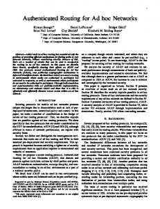
3.1 Augmented Route Tree for OOC, SOC and Crankback Control Rules

27

3.2 Queueing model for processing delay and call holding times : : : : : :

33

3.3 Equivalent queueing model for processing delay and call holding times 34 3.4 Augmented Route Tree for OOC Control Rules (homogeneous case). :

35

3.5 Routing tree for SOC and Crankback control rules (homogeneous case) 39 3.6 NSFNET topology : : : : : : : : : : : : : : : : : : : : : : : : : : : :

46

3.7 Simulation results vs analysis results : : : : : : : : : : : : : : : : : :

48

3.8 Comparison of dierent routing schemes : : : : : : : : : : : : : : : :

49

3.9 The eects of processing delay and admission control function. : : : :

51

4.1 Applying Markov decision process to the simpli ed link model: single class of trac. : : : : : : : : : : : : : : : : : : : : : : : : :

75

4.2 Applying Markov decision process to the simpli ed link model: multiple classes of trac. : : : : : : : : : : : : : : : : : : : : : : :

76

4.3 A simple network for investigating the eect of link independence assumption : : : : : : : : : : : : : : : : : : : : : : : : : : : : : : :

86

5.1 Example: A 5-node network and its corresponding VP network. : : :

97

5.2 Example: A simple VP network : : : : : : : : : : : : : : : : : : : : : 101 5.3 Comparison of the maximum number of VC's that can be supported under dierent cell control schemes. : : : : : : : : : : : : : : : : : 106 5.4 Maximum number of VC's that can be supported under the ADAPTIVE scheme. : : : : : : : : : : : : : : : : : : : : : : : : : 108 5.5 Performance of dierent routing policies : : : : : : : : : : : : : : : : 123

xiii

CHAPTER 1 INTRODUCTION In computer networking, major research activities have always been preceded by signi cant advances in the underlying communication technology. For example, research in packet-switching networks during the 1970s and 1980s was preceded by major advances in processors (store-and-forward switches) and communication technologies. In the 1990s, signi cant advances in ber optic and switching technology have precipitated the current explosion in the amount of research in future high-speed networks. The challenges facing high-speed network researchers result not just from the high data transmission rate but also from other new characteristics not previously encountered in traditional circuit-switched or packet-switched networks. For example, features such as large propagation delay as compared to transmission delay, diverse application demands, constraints on call processing capacity, and quality-of-service (QOS) support for dierent applications all present new challenges which arise from the new technology and new applications. Thus, much research is needed not just to improve existing technologies, but to seek a fundamentally dierent approach toward network architectures and protocols. In particular, new ow control and routing algorithms need to be developed which account for these new network characteristics. The goal of this dissertation is to solve routing problems in the context of highspeed networks taking into account the new network environment. In order to better understand the in uence of these new network characteristics on the routing problem, we rst study the computational delays associated with call admission, routing and call setup in future high-speed networks. This study also leads us to explore the similarity between call setup in high-speed networks and circuit-switched networks and to study how approaches toward routing in circuit-switched networks can be adapted for routing in high-speed networks. Speci cally, based on the Markov

2 Decision Process (MDP) framework, we next design and evaluate state-dependent routing algorithms for high-speed networks which account for these new network characteristics. Finally, we consider a Virtual Path (VP) concept that has been proposed to simplify trac control and resource management in future high-speed networks. Thus, in the last part of this dissertation, we also demonstrate the eciency of MDP-based routing algorithms in virtual path-based networks.

1.1 Problem Formulation In this dissertation, we will rst examine the in uence of the characteristics of high-speed networks on the routing problem. We then design and evaluate routing algorithms to account for these new features. In the rst part of this dissertation, we focus on the computational delays associated with call admission, routing and call setup in future high-speed networks. Although the CCITT speci cations on ATM [17] specify a cell-based, packet-like transport mode for information within the network, the need to provide a guaranteed QOS has resulted in the need for a call-level admission control mechanism and the reservation of resources (e.g., bandwidth [2]) by a call on a link-by-link basis. Thus when a call is \oered" to a route, computations will be required at each node on the route in order to determine whether the selected route can indeed support the additional call while meeting the QOS guarantees already made to existing calls. In future high-speed networks, signi cant burdens will therefore be placed on the processing elements in the network and the bottlenecks are likely to shift from the communication links to the processing elements. The processing delays at these processing elements are in uenced by network parameters such as the routing algorithm used, propagation delays, admission control functions (due to QOS requirements), path lengths (or network topology), and processing capacities at these elements. The goal of this research is to characterize the in uence of these network characteristics on the call setup time and accepted call throughput. In chapter 3, we will develop analytic models for evaluating the average call setup time and accepted call throughput for various routing algorithms.

3 The need to reserve resources such as buer space and bandwidth for each individual connection in order to guarantee its QOS requirement has made connection establishment in high-speed networks quite similar to call setup in circuit-switched networks. Thus in the second part of this dissertation, we develop adaptive routing algorithms for high-speed networks based on routing algorithms previously developed for circuit-switched networks. Adaptive routing algorithms in circuit-switched networks can be classi ed into two categories: Least-Loaded Path-based (LLP) and Markov Decision Process-based (MDP). Three problems can be identi ed in applying these routing algorithms to high-speed networks. First, most routing algorithms assume the existence of a \direct link" between every O-D pair and use that link as the primary path. This may not be a reasonable assumption in high speed networks. Second, while MDP routing algorithms yield very promising performance in single class circuit-switched networks, they become too computationally expensive in multiclass networks. An approach is thus needed which can reduce this computational complexity if we are to apply Markov decision theory to routing problem in high-speed networks. Finally, in order to make the analytical model tractable, MDP routing algorithms make a link independence assumption. Such an assumption is acceptable in circuit-switched networks because of their densely connected topologies. However, as the network topology becomes increasingly sparse, the states of the links in the network become increasingly correlated. Since we expect that future high speed networks will indeed be very sparse, it is questionable whether applying MDP routing algorithms from circuit-switched networks to future high-speed networks can still yield good performance. We will address these issues in chapter 4. In the last part of the dissertation, we study the routing problem in Virtual Path networks. In order to facilitate trac control and resource management in future high-speed networks, a Virtual Path (VP) concept has been proposed [18, 21, 73]. A VP can be viewed as a logical direct link between a source node and a destination node which physically consists of a set of adjacent links. By reserving \capacity", e.g., bandwidth and buer space, on VPs, the call establishment processing can be simpli ed signi cantly because a call acceptance decision can immediately be made at the source node (without the need for a hop-by-hop call set up). However, this

4 advantage is oset by the increase in network blocking probability because of the statistical multiplexing gains lost by the preallocation of capacity to the virtual paths. Thus, there exists a trade-o between the call setup cost and the call blocking probability. Two approaches can be used to reduce the network blocking probability when bandwidth is reserved for virtual paths. The rst approach is to logically view the network as a fully connected network with virtual paths serving as links in the virtual network. Adaptive routing algorithms based on Markov decision theory can then be used to reduce the blocking probability. The second approach is to have a dynamic virtual path bandwidth allocation algorithm which can reduce the call set up delay signi cantly while maintaining a competitive call blocking probability. In chapter 5, we will focus on the rst approach and develop and evaluate adaptive MDP routing algorithms and virtual path bandwidth reservation schemes for networks with reserved virtual path bandwidth.

1.2 Research Contributions The goal of this dissertation is to characterize the in uence of new network characteristics introduced by high-speed networks on the routing problem and to develop and evaluate appropriate approaches toward routing in such networks which account for these new features. Below, we list our important contributions in the order in which they appear in this dissertation. We rst study the in uence of new network characteristics introduced by highspeed networks on the routing problem. Our contributions in this study include: The development of analytic models for evaluating the average call setup delay and accepted call throughput for three sequential routing algorithms and two

ooding routing algorithms. These analytic models are more comprehensive than those introduced in previous works on routing in the literature in that propagation delay, call setup delay, blocked call clear time and processing delay are explicitly modeled.

The examination, through analytic models, of the eect of call processing delay,

propagation delay, admission control function, and routing algorithms on the average call setup delay and call throughput.

5

The observation that the average call setup delay and call throughput are very sensitive to that call processing service time, admission control function, and routing algorithm, but are relatively insensitive to the propagation delay.

The great similarity between routing in circuit-switched networks and high-speed networks has inspired us to examine and apply adaptive routing algorithms in circuitswitched networks to high-speed networks. We focus on designing and evaluating adaptive routing algorithms for future high-speed networks based on Markov decision theory. The contributions of this study are listed below:

We propose and evaluate an LLP-based routing algorithm for high-speed networks.

We propose an approach for computing approximate link shadow prices for

multi-class networks which is computationally feasible while still providing quite accurate routing information.

Based on the approximate link shadow prices, we design and evaluate various

MDP-based routing algorithms, and show that they outperform the LLP-based routing algorithm.

From a simple network model, we have found that the performance of MDP-

based routing algorithms is insensitive to the validity of the link independence assumption.

In the last part of this dissertation, we study the routing problem in VP networks. Our contributions in this work are listed below:

We explore two strategies for reserving VP capacity: a deterministic strategy

and a statistical strategy. We also examine advantages and disadvantages of these two strategies. We show that routing policies are able to yield signi cantly lower blocking probability when the statistical reservation strategy is adopted.

We design and evaluate MDP routing algorithms for homogeneous VP networks

and show that MDP routing algorithms are able to provide signi cantly lower network blocking probability with slightly increase in control cost.

6

We propose a VP capacity sharing concept in which some VPs are allowed to

borrow capacity from other VPs. We also design MDP routing algorithms which account for this concept and show that routing algorithms which account for the VP capacity sharing concept are able to further reduce the network blocking probability.

1.3 Overview of the Dissertation The remainder of the dissertation is organized as follows. We rst brie y review, in chapter 2, existing routing algorithms for both circuit-switched and packet-switched networks. We also examine a commonly-used analytic technique for evaluating call blocking probability in circuit-switched networks. We then discuss some new network characteristics introduced by new technologies and applications and challenges posed on the routing problem in future high-speed networks. In chapter 3, we examine the in uence of these new network characteristics on routing. This in uence is examined, through analytic models, with three sequential routing schemes and two ooding routing schemes under various network parameters and dierent forms of admission control. Chapter 4 applies adaptive routing algorithms from circuit-switched networks to high-speed networks. In particular, we focus on developing computationally feasible MDP routing algorithms for high-speed networks. We also examine the eect of the link independence assumption on the performance of MDP routing algorithms. While chapter 4 deals with networks without the VP concept, chapter 5 deals with VP networks. In this chapter, we design and evaluate MDP routing algorithms under dierent virtual path capacity reservation strategies for \homogeneous" VP networks, i.e., VP networks with homogeneous trac sources. Finally, chapter 6 summaries this dissertation and suggests directions for future work.

CHAPTER 2 AN OVERVIEW OF ROUTING In this chapter, we rst brie y review existing routing algorithms used in both circuit-switched and packet-switched networks. There are three categories of routing algorithms: static routing, adaptive routing and dynamic routing [39]. In static routing, all routing decisions are made at network setup time and are xed, independent of the network state. Dynamic routing allows routing decisions to vary over time, but not necessarily depend on the network state. Finally, in adaptive routing, routing decisions are based on a function of some estimate of the network state and thus may also vary over time. The dierence between dynamic routing and adaptive routing is that an adaptive routing algorithm usually is also dynamic unless the network is so quiet that the network state is not changing at all. However, the converse is not necessary true. Especially in circuit-switched networks, some algorithms, e.g., Dynamic Non-Hierarchical Routing in AT&T's long distance network, change their routing decisions at xed time intervals, but do not use network state measurements. This chapter is structured as follows. The rst section reviews existing routing algorithms used in circuit-switched networks. It also examines a commonly used analytic technique for evaluating the performance of a circuit-switched network. Routing algorithms used in wide-area packet-switched networks are brie y discussed in the second section. We are not interested in routing algorithms in LAN's and MAN's because they are relatively simple due to the special structure of network topology, e.g., bus, loop, ring and tree. In the last section, we discuss some new characteristics introduced by new technologies and applications and the resulting challenges posed by the routing problem in future high-speed networks. This section concludes with a list of the characteristics of the routing problem in high-speed networks.

8

2.1 Routing in Circuit-Switched Networks In a circuit-switched network, a call setup procedure is used to set up a dedicate, end-to-end, connection between users who desire to communicate. The routing algorithm provides the rules which a call setup procedure follows for each connection request. When a call arrives, the call setup procedure rst chooses a path (a sequence of links from the origin node to the destination node) from a set of possible paths according to the routing algorithm and then proceeds as follows. First, the origin node passes the call request to its downstream neighbor on the chosen path. If the neighbor, \successfully" receives the request, it then passes it to its downstream neighbor on the path. This transfer of the call request from one node to another is \successful" if there is at least one free circuit in the link connecting these nodes that can be reserved for the call. This process continues until either the request is successfully passed to the destination node or the request cannot be passed further towards the destination node by an intermediate node on the path. In the rst case, the call is established and the circuits reserved along the path by the call setup procedure provide a private, end-to-end connection. In the second case, the call cannot be established on the path and, depending on the routing algorithm, a \blocking" message needs to be sent back either to the upstream node or all the way back to the source node. Three methods have been proposed for responding to a blocking message. The rst method is called originating-oce control (OOC). Under OOC, the blocking message is transmitted all the way back to the origin node and all circuits that have been reserved are released. When the blocking message is received, the origin node chooses the next path from the set of all possible paths and repeats the procedure described above. The second method is called sequential-oce control (SOC), also called progressive control, sequential control, or spill forward without crankback, in which the intermediate node chooses the next outgoing link to try when a blocked link is encountered. In this case, no blocking message is fed back to upstream nodes and a call is blocked only when all the possible outgoing links of an intermediate node (or the origin node) are blocked. If this occurs, the circuits reserved on the path to the node are released and the call is aborted. The third method is called crankback, or spill forward with crankback. The only dierence between the SOC

9 method and crankback method is that with crankback, a blocking message is fed back to the upstream node when the downstream node is blocked. A node is blocked if all of its possible outgoing links (for the O-D pair) are blocked and a call is blocked if the origin node is blocked. If a blocking message is fed back to the upstream node, the circuit reserved on the link from the upstream node to the node is released. A detailed survey of existing routing algorithms for circuit-switched networks is given in [49]. We brie y list below some well known routing algorithms. The oldest and most extensively used static routing algorithm in telephone networks is the hierarchical alternate routing algorithm [9, 76]. Because of the ineciency of static routing, a dynamic routing algorithm, Dynamic Non-Hierarchical Routing (DNHR), was introduced in the long distance AT&T network in the United States in the mid 1980s to replace the old hierarchical alternate routing algorithm [7]. Another dynamic routing algorithm is Dynamic Alternate Routing (DAR) which has been proposed for the British Telecom's domestic network. Both DNHR and DAR oer a new arriving call to the direct link rst. If it is blocked, alternate paths are tried. In DNHR, a day is typically divided into 10 periods of time and a near-optimal alternate routing sequence is computed o-line for each period. As each time period starts, the appropriate routing table is selected. Calls that are blocked on the direct link are oered to the alternate paths according to the prede ned order in the routing table. In DAR, the origin switch keeps a recommended alternate path. A new arriving call that is blocked on the direct link is oered to the recommended alternate path only. If the recommended alternate path is busy, the call is blocked and a new recommended alternate path is selected randomly from the set of possible alternate paths. Otherwise, the call is set up on the recommended alternate path and the recommended alternate path remains unchanged. Since the mid 1980s, considerable research has focused on the design of adaptive routing algorithms for circuit-switched networks. Existing adaptive routing algorithms can be classi ed into two categories: Least-Load Path-based (LLP-based) and Markov Decision Process-based (MDP-based). The LLP approach tries to route calls to the \least busy" path, i.e., the path that has the maximum free circuits. The MDP approach, on the other hand, formulates the routing problem as a Markov

10 decision process. LLP-based routing algorithms include AT&T's Trunk Status Map Routing (TSMR) [6] and Real-Time Network Routing (RTNR) [8], and Bell-Northern Research's Dynamically Controlled Routing (DCR) [71, 81]. MDP-based routing algorithms include Bellcore's State-Dependent Routing (SDR) [56] and Forward-Looking Routing (FLR) [58], and routing algorithms based on INRS-Telecommunications' Markov Decision Process Decomposition (MDPD) approach [29, 31, 32, 33].

2.1.1 Performance Evaluation The most important performance measure for circuit-switched networks is the call blocking (or loss) probability, either the loss probability of an origin-destination pair or the loss probability of the network over all O-D pairs. Thus, minimizing the call blocking probability is the most common objective of routing algorithms in circuit-switched networks. A rather simple, explicit method for computing call blocking probability is to make appropriate assumptions, model the system as a Markov process, and compute the blocking probability. However, this quickly yields a very large state space as the complexity of the network and the capacity of the links grow. On the other hand, with the assumption of Poisson arrivals at each link, the individual link blocking probability can be computed easily and quite accurately by the well-known Erlang's B formula provided that the link-oered trac (i.e., the mean call arrival rate of the arrival process at the link) and link capacity are known. After the blocking probability of each link is computed, the overall network performance can be computed based on these measures. This idea yields the link-decomposition method [39], a simple and commonly used method for evaluating the call blocking probability for circuitswitched networks. The link-decomposition method is based on the following assumptions: 1. External call arrivals are assumed to be independent, stationary Poisson processes. 2. There is no blocking at the switches. 3. Calls are blocked independently at all links.

11 4. Calls that cannot be routed on a path are cleared in zero time, and are returned to the responsible switches in zero time, if necessary. 5. The network topology is xed, routing decisions are given, and are not allowed to change during the calculation. 6. Call holding times are independent and identically distributed, and are usually assumed to be exponentially distributed, but not always. (e.g. in [53, 82], call holding times are arbitrarily distributed.) The diculty with this method arises from the fact that the link-oered trac is unknown and coupled with the link-blocking probability. That is, on one hand, we need to use the link-blocking probability to compute the link-oered trac. On the other hand, we need the link-oered trac to compute the link-blocking probability. This yields a xed point problem which in most cases, is solved by an iterative method consisting of the following two stages: 1. Given the link-blocking probabilities, one can compute the link-oered trac and call-blocking probabilities. This computation depends on the routing algorithm used. 2. The resulting link-oered trac in turn yields, via the Erlang-B formula, a new set of values for the link-blocking probabilities. When an iterative method is used to nd a solution, one may ask if a unique solution exists. Since the two stages can be viewed as a continuous mapping from (0; 1)` to itself, where ` is the number of links in the network, and the possible solution set is bounded by (0; 1)` , one can use the classical Brouwer xed-point theorem to prove that there exists at least one xed point. Then, under some sucient conditions, this mapping can be proven to be a contraction mapping, and therefore yielding a unique solution. However, the sucient conditions are usually very strong (e.g., [82]). Furthermore, there is no guarantee that the iterative method will nd a solution, even if one exists [39]. We will discuss the convergence problem in more detail after we review some related previous works.

12 In [82], Whitt proposes a model for calculating the blocking probability in setting up virtual circuits in packet-switched networks. The model, called reduced-load approximation, is very similar to the link-decomposition method. In [82], alternate path routing is not considered, i.e., every virtual circuit has only one path to try, and is lost if it is blocked at any link of the path. All resources required by a virtual circuit are seized and freed together. Poisson arrival processes and general service distribution are assumed (M/G/s/loss), although Whitt indicates how to apply the reduced-load approximation to a single facility (link) with non-Poisson arrival processes. Whitt has proved that the approximate link-blocking probabilities can be bounded above and below, and very often these upper and lower bounds will converge. However, the exact link-blocking probabilities are not necessarily bounded by these bounds. He also shows that under some very strong conditions the iterative method has a unique solution. Kelly in [53] applies this model to circuit-switched networks and proves that this model always has a unique solution, the so called Erlang xed point. Kelly also shows that the approximate solution is asymptotically exact in heavy trac. Yee [84] develops a model in which SOC routing is used and the procedure for choosing the next node through which to set up a call is rather complicated. In his model, each node has multiple permutations of downstream adjacent nodes for each call set up request to be selected as the next node. The choice of a permutation is determined by a prede ned probability. The link-decomposition method is used to transform the model into a set of nonlinear equations. He proves that, under certain conditions, the system has a unique solution by showing that the nonlinear transformation is a contraction mapping. The nonlinear equations formulated by Whitt, Kelly and Yee are rather simple because they only consider xed routing or SOC routing. When OOC routing and crankback routing are used, a complication arises, due to the fact that some links can appear on more than one path (place) in the same routing tree. This fact complicates the computation of the probability that a call will be routed through a particular path. The reason is that if some link on the path appears on some other path before the one considered, the probability that the path is free and the probability that the

13 call over ows to this path are not independent. This is true even if we assume that the individual link-blocking probabilities are independent. The problem arises from the assumption that blocked calls have zero holding time, so if a given link blocks a call on one path that link blocks all calls on all paths to which it belongs. As a consequence, the probability that a call will be routed through a particular path is a conditional probability. Butto, Colombo, and Tonietti [15] rst propose a complete analysis for OOC routing for the case in which a link may appear more than once in a given routing tree. Links that appear more than once in a tree are called repeated links. The probability of routing a call through a particular path is computed by explicitly considering all of the possible combinations of states of all the repeated links, where the state of a repeated link is either free or busy. It is easy to see that the state space grows exponentially in the number of repeated links. They also formulate a model for SOC routing and observe that it is not necessary to compute conditional probabilities when calculating the probability of using a particular path. This is because the probability of using a particular path is independent of whether a link on the path appears elsewhere in the routing tree when SOC routing is used. In parallel with [15], Lin, Leon, and Stewart [59] propose an analysis method for computing the end-to-end blocking probability for OOC, SOC, and OOC with spill-forward routing strategies. (OOC with spill-forward is a combination of OOC and SOC routing.) Repeated links are also considered. The probability of using a particular path is calculated by examining the sequence of all paths speci ed by the routing strategy, the so called path-loss sequence (which is generated by hand). An iterative procedure is used to solve the non-linear equations. However nothing is mentioned regarding whether the procedure will nd a solution, or even if a solution exists. The diculty of generating the path-loss sequence in [59] is solved by Chan [22]. Chan develops a recursive algorithm for computing the end-to-end blocking probability for an arbitrary routing tree by recognizing the underlying recursive nature of the problem. The main idea is to compute the link set, a set containing links that appear in previous paths but not in current path, recursively. The importance of this

14 work is the use of recurrence relations which makes the calculation applicable to all static routing strategies with alternate routing. The complexity of the recursive algorithm in [22] cannot be polynomially bounded. This is due to the nature of the problem. Girard and Ouimet [40] propose a recursive algorithm that can be polynomially-bounded for a routing tree in which there are no repeated links. The result is not surprising because the complexity of the problem in [22] comes from the fact that they consider arbitrary trees with repeated links. In parallel with Chan's work, Gaudreau [36] also proposes a recursive formula for calculating the end-to-end blocking probability for SOC routing with a xed sequence route selection at each node. The computation is based on the assumption that the individual link blocking probabilities are known and independent. The repeated links cause no complication in the computation, as explained above. Algorithms presented in [15, 59, 22, 40, 36] describe how the end-to-end blocking probability can be computed, given the individual link blocking probabilities. Only [40] and [59] show how to compute the individual link blocking probability. Girard and Ouimet [40] further show that the computation of the appropriate link blocking probabilities is best done by a xed point method, rather than a Newton-type algorithm, because the amount of computation required by the latter algorithm is too high. Unfortunately, there is no guarantee that the xed point method will nd a solution, even if one exists [39]. Moreover, Akinpelu's work in [4] indicates that the existence of more than one solution arises in connection with real instabilities in networks operating with nonhierarchical alternative routing. Recall that this undesirable phenomenon does not happen in Kelly and Yee's work [53, 84]. It therefore seems that this phenomenon is closely related to the nature of OOC routing (crankback routing has never been explored by this kind of analysis). Theoretically, some very strong sucient conditions can be imposed that guarantee a unique solution.

2.2 Routing in Packet-Switched Networks In a packet-switched network, the function of the routing algorithm is to select the best set of available links to transfer a packet between a source and destination. In the broadest sense, two approaches towards routing may be identi ed. They

15 are distinguished by the times at which routing decisions are made. In a virtual circuit network, a routing decision is made when each virtual circuit (VC) is set up. The routing algorithm is used to choose an end-to-end path for the VC. All packets belonging to the VC subsequently traverse the network following this path and arrive at the destination node in the sequence in which they were transmitted. This VC routing approach embodies the so-called \connection-oriented" approach towards packet-switching. The second approach towards routing is a connectionless one, with packets (datagrams) moving through the network on an individual basis, with a routing decision being made for each individual packet. The issue of whether a datagram or VC approach is a better choice for a packet switching network has been debated for a long time. The advantages of datagram routing include the provision of robust service in the face of network component failures and the exibility of building dierent types of services on top of it. But congestion control and the requirement of resequencing for some applications are serious problems for datagram networks. On the other hand, virtual circuit networks provide easier congestion control and no need for resequencing; these are provided at the cost of explicit call set up overhead and a vulnerability to network component failures. In terms of performance, Rudin in [72] notes that the delay in a network that assign routes on a session basis is less than that in a system that adapts the route more frequently when the network is protected by ow control and the network load is reasonable high. Finally, it should be noted that most of the high-speed network designs for the future are clearly directed toward connection-oriented or partially connection-oriented approaches. The objective of routing in packet-switched networks is to obtain a high network throughput while keeping the average packet delay as low as possible. (Unfortunately, operating any queueing system near capacity implies a long queueing delay.) Throughput and average packet delay are the two important performance measures that are substantially aected by the routing algorithm. Routing interacts with ow control in determining these performance measures [12]. The eect of good routing is either to (a) increase the throughput as high as possible for the same value of average delay per packet under high network load or (b) decrease the average packet delay for the same level of network throughput under low network load.

16 During the last three decades, many routing algorithms for wide area networks have been proposed. A survey of those routing algorithms is given in [49]. In this survey, due to the great diversity in existing sophisticated adaptive routing algorithms, adaptive routing algorithms are further classi ed according to the following two ways. First, according to the route selection mechanism, adaptive routing algorithms are further classi ed into shortest-path-based algorithms and gradient-based algorithms. Second, according to the method of information dissemination, adaptive algorithms are further classi ed into centralized, isolated, and distributed algorithms. Although research in adaptive routing in packet-switched networks is quite successful, in the next section, we will show that these adaptive algorithms are not suitable for high-speed networks.

2.3 Routing in High-Speed Networks In this section, we rst examine four new network characteristics introduced by the new technology and new applications of future high-speed networks and discuss how they aect the routing problem. We then discuss how these characteristics make routing in future high-speed networks similar to, as well as dierent from, the routing in both circuit-switched and packet-switched networks. Finally, we conclude this section by listing characteristics of routing in high-speed networks.

2.3.1 New Characteristics of High-Speed Networks Very limited processing capacity:

In the last decade, network transmission rates have increased by at least four orders of magnitude while processing capacities have only increased by two orders of magnitude. The result of this change is that the time available to process a packet at an intermediate node is very limited [60]. Thus implementing complicated datagram routing algorithms in high-speed networks may not be feasible. In other words, virtual circuit routing will be better suited for future high-speed networks. For example, CCITT has recommended that the ATM networks be connection-oriented [17].

17 The very limited processing time for each packet leads to a need for developing a dedicated hardware switch that has the ability to route packets very quickly, without consuming the processing capacity [26]. According to [26, 25], this can be achieved by building a network node in two parts: the switching subsystem (SS) and the Network Control Unit (NCU). The SS is a fast hardware switch with relatively limited functionality. The NCU is a slower but more sophisticated processor. Packets that are only relayed through the node, e.g., control packets in a virtual circuit, are handled by the SS directly without involvement of the NCU. Packets that require more complex processing, e.g. packets that carry call set up and routing information, are forwarded from the SS to the NCU. Source routing, where every packet carries its own path information, is also recommended in [26, 25] so that packets can be quickly switched by the SS at transit nodes. Although processing requirements can be decreased by doing virtual circuit routing and switching normal packets via a switching subsystem, signi cant burdens will still be placed on the processing elements in future high-speed networks since call routing and admission control will be computationally intensive. Thus the processing elements in high-speed networks are very likely to become a new bottleneck.

Long relative propagation delay:

When transmission rates and processing capacities both increase by at least two orders of magnitude, the propagation delay does not change. It has been shown that delays at the switches are less than 1% of the total end-to-end delay [10, 85]. It is thus obvious that propagation delay forms a major component of average packet delay in a high-speed wide area network. This has a big impact on current existing adaptive routing algorithms in the following two ways: 1. For shortest-path based routing algorithms, the link lengths are mostly determined by the measured delay on the link. Since the propagation delay contributes 99% of the delay, the measured link delay is almost always equivalent to the propagation delay. In other words, the delay on the

18 link is not signi cantly aected by trac changes unless the load is very high. For gradient-based routing algorithms [12, 35], the cost function for optimization is also a function of propagation delay and queueing delay. Similar to the shortest-path based routing algorithms, the gradient-based routing algorithms are also very likely to route all virtual circuits to the path with shortest propagation delay. 2. For adaptive routing algorithms (centralized or distributed), information collected at individual nodes needs to be passed to decision point(s). The quicker the information is received, the better the performance of the routing algorithm. When the propagation delay is much larger than the packet transmission time, the information received by the decision point(s) may be too old to use [37]. Another consequence of long propagation delays is that the number of packets in transmission media becomes very large so that the ability to do source-based (or feedback-based) ow control decreases. The validity of traditional windowbased ow control mechanisms in high-speed future networks is questionable. Rate-based ow control mechanisms are believed to be more appropriate for the future network [28, 64, 86].

Support of diverse services:

Another challenge of high-speed networks is the need to support a wide variety of applications with stringent and diverse service requirements. Examples are le transfer, real-time packet voice, teleconferencing, high-resolution graphics, computer visualization, and remote procedure calls. Applications such as conventional le transfer require high reliability, while applications such as real-time packet voice, teleconferencing, and remote procedure calls require short network delay as a primary consideration. Applications such as high-resolution graphics and computer visualization require a signi cant amount of bandwidth while others, such as remote procedure calls, require only a very small amount of bandwidth.

19

Support of quality of service:

One of many interesting challenges facing future high-speed networks is how to provide Quality-Of-Service (QOS) support for dierent classes of applications. The QOS requirement of a connection with respect to loss probability, end-to-end delay, delay jitter, has to be negotiated with the network at call set up time. The QOS requirements clearly aect (and are aected by) both routing and

ow control [86]. In routing, an admission control function is invoked at each link on the route being examined to decide whether the new connection can be accepted or not. The decision has to be made based on the incoming call's trac characteristics, the QOS requirements of the new connection, and all the existing connections sharing part or all of the same network resources. Acceptance occurs only if the QOS requirements can be achieved for all connections concerned (i.e., the newly arriving call and the already accepted calls). The objective of the admission control function as well as the routing algorithm is to accept as many new connections as possible while still guaranteeing the QOS requirements for every existing call. Due to the statistical multiplexing nature of packet-switched networks, call admission may not be sucient for providing QOS guarantees to all accepted calls because the actual trac of a connection may deviate from its negotiated trac characteristics. Therefore, it is necessary to introduce a new congestion control function, the so called \policing" function, to restrict the behavior of each trac source to the characteristics negotiated in order to prevent the degradation of the QOS for all connections. The in uence of this characteristic on routing is that some connection-oriented performance metrics, such as average packet delay or packet loss probability, which used to be part of the cost function to be optimized by routing in traditional packet-switched networks now becomes a constraint to be satis ed when routing in high-speed networks. Other design goals, such as minimizing processing requirements, average call set up time, or maximizing the number of accepted calls, will become the new objective of routing [3, 10].

20

2.3.2 Comparison of Routing in High-Speed Networks with Routing in Traditional Networks Similarities and dierences between call set up in high-speed networks and circuit-switched networks

The need for admission control to support QOS requirements has made connection establishment in high-speed networks very similar to call set up in circuitswitched networks. In circuit-switched networks, a call is successfully established on a route if each link on the route has at least one nonbusy circuit. On the other hand, the need to provide a guaranteed QOS in high-speed networks has resulted in the need for a call-level admission control mechanism and the reservation of resources (e.g., bandwidth [2]) by a call on a link-by-link basis. Thus in high-speed networks, a new connection is accepted if and only if, for each link on the route, adding the new connection will not violate the QOS requirements of all existing connections sharing the same link. In the case that a new call (connection) is rejected along the route under investigation, the routing functions in both types of network need to select, if possible, another route between the same source and destination node to try to set up the call. The fundamental dierence between high-speed networks and circuit-switched networks is that high-speed networks are expected to be packet-switched networks. For example, the Asynchronous Transfer Mode (ATM) standard that has been designated for the future high-speed networks is packet-oriented [62]. Packet switching has many advantages, such as providing higher bandwidth utilization, more exible multiplexing of diverse services with dierent bandwidth requirements, and taking advantage of statistical multiplexing gains among services. Given that high-speed networks will be packet-switched, the call (connection) set up in circuit-switched networks and high-speed networks dier at least in two aspects: 1. The criteria (admission control function) to determine whether a link can accept a new call is very dierent, i.e., no free circuits (in the circuit-switched

21 case) vs. some complicated function of trac characteristics of existing and new connections (in the packet-switched case). 2. In circuit-switched networks, a dedicated (unshared), end-to-end connection is provided to each call, while this is not necessarily true in high-speed networks. High-speed networks may be engineered to take advantage of statistical multiplexing gain among dierent services while still guaranteeing QOS requirements for every service.

Similarities and dierences between call set up in high-speed networks and packet-switched networks

Although high-speed networks are expected to be packet-switched, the method for establishing a new connection (virtual circuit) will be very dierent from that in traditional packet-switched networks. In traditional packet-switched networks, QOS is not provided and no admission control is used in setting up a virtual circuit. In most cases, congestion control has not been a concern of the routing algorithm. That is, a virtual circuit will not be rejected by the routing algorithm in a traditional packet-switched network unless there is no physical path from source to destination. The objective of routing is to route every virtual circuit (or datagram) on the best path according to current available information. (This is the so called \best-eort" delivery strategy.)

With QOS requirements, routing in high-speed networks cannot use such a \besteort" delivery strategy. A new connection needs to be rejected if its acceptance will prohibit the network from providing the negotiated QOS for all existing calls. Moreover, among the paths that can accept the new connection, the path that has the expected minimum packet delay or loss probability need not be the best path to choose under a new optimization criteria such as maximizing the total number of connections accepted by the network. Still another dierence is, as mentioned above, that routing in high-speed networks needs to attempt call setup on other possible routes when a call is rejected by the route under investigation; there is no such \blocked route" in traditional packet-switched networks.

22

2.3.3 Characteristics of Routing in High-Speed Networks It should be clear that routing in high-speed networks has elements of routing in both circuit-switched and packet-switched networks, but that it also signi cantly diers from both. From our previous discussion, we can conclude that the future high-speed networks are expected to be connection-oriented networks, supporting multiple classes of QOS requirements. Thus routing in future high-speed networks is expected to be virtual circuit-oriented with the following constraints: 1. A connection is accepted on a route only if for each link on the route, adding the new connection will not violate the QOS requirements for all existing connections sharing the same link. 2. Due to the long propagation delay, global network status information is either unavailable or obsolete. Furthermore, the objective of routing is to: 1. Maximize the total number of connections admitted to the network under some form of fairness constraint. 2. Minimize the average call set up time which includes processing time and queueing delay at each node (switch) visited, and propagation delay at each link traversed. Maximizing the network throughput (in this case, the total number of connections admitted) has always been the primary objective in designing a routing algorithm in the past. It will remain the primary objective for routing algorithms in future highspeed networks. In traditional packet-switched networks, another objective would be to minimize the end-to-end packet delay. In future high-speed networks, end-to-end packet delay may be not the concern of all applications and in the case that it is the main concern of the application, the end-to-end packet delay for each packet (or certain percentage of the packets) can be guaranteed according to the application's requirement by appropriate network resources management (e.g., scheduling policy, buer management, etc). On the other hand, because of the long propagation delay

23 and processing delay (as compared to the transmission delay), the call setup delay will become an issue. Thus minimizing the call setup time will be a desirable objective in designing routing algorithms for future high-speed networks.

CHAPTER 3 THE INTERACTION OF CALL PROCESSING DELAYS AND ROUTING IN HIGH-SPEED NETWORKS In order to ensure that accepted calls will be provided with a guaranteed QOS, signi cant burdens will be placed on the processing elements in future high-speed networks. The need to provide a guaranteed QOS has resulted in the need for a call-level admission control mechanism and the reservation of resources (e.g., bandwidth [2]) by a call on a link-by-link basis. In this latter case, when a call is \oered" to a route, computation is required to determine whether the selected route can indeed support the additional call while continuing to meet the QOS guarantees of existing calls. The manner in which calls are oered to the various routes (e.g., the order in which routes are attempted and the decision as to whether multiple call setup paths will be attempted in parallel) will clearly in uence the call setup time as well as the maximum call arrival rate that can be supported by the network call processing elements. Network parameters such as call processing capacities, propagation delays, and path lengths will also in uence these performance measures. We seek to characterize the in uence of these routing, call setup, and network characteristics on the call setup time and the accepted call throughput in this chapter. This chapter is organized as follows: in section 3.1, we discuss our model of the network. In section 3.2, we specify the routing mechanisms examined. Section 3.3 contains the analytical models for dierent routing mechanisms. The results of our investigation on the in uence of processing delay, admission control function, and routing algorithms on the average call setup delay and accepted call throughput are presented in section 3.4. The in uence of propagation delay on routing, presented in [51], is summarized in section 3.5. Section 3.5 also discusses the issue of whether it is important to model resources held by blocked calls. Finally, section 3.6 summarizes this chapter.

25

3.1 Network Model We consider a connection-oriented high-speed network consisting of N nodes, N 2, with each node having some number of incoming and outgoing links. We adopt the network node structure described in [25, 26], in which a node consists of two components: the switching subsystem (SS) and the network control unit (NCU). The SS is a fast hardware switch with relatively limited functionality. The NCU is a slower, but more sophisticated, processor. Packets (or cells) that need only be relayed through the node are handled by the SS directly without the involvement of the NCU. We further assume that control packets associated with routing are the only control packets processed by the NCU. Each NCU is assumed to have a suciently large buer to avoid the loss of routing control packets due to buer over ow. External connection requests, each having an associated QOS requirement, can arrive at any node in the network. When a call request arrives, the routing algorithm (which resides in the NCU's of the network nodes) chooses a path for the call from a set of possible paths (according to the rules speci ed in next section) and then proceeds as follows. First, the source node invokes the admission control function to check if the new call can be accepted on the rst link on the path. The call is accepted on the link if sucient bandwidth is available on the link to meet the new call's QOS requirement, while maintaining the agreed-upon QOS for existing calls. If the call is accepted on the link, a certain amount of the bandwidth, determined by the QOS requirement, is reserved for the call. The source node then passes the call request to its downstream neighbor on the chosen path. This neighbor then passes the call request to its downstream neighbor if the QOS can also be guaranteed at the next link. This process continues until either the request is successfully passed to the destination node or the request cannot be passed further toward the destination node by an intermediate node on the path. In the rst case, the call is established and the resources reserved along the path during the call set-up phase provide the guaranteed QOS required by the call. In the second case, the call cannot be established on the path, bandwidth that has been reserved for this call is released, and another path, if available, may then be tried.

26

3.2 Routing Algorithms We examine the eects that ve routing algorithms, three sequential algorithms and two controlled- ooding algorithms, have on the call setup time and accepted call throughput. We assume that for each source-destination pair, there is a prede ned routing tree available at the source node [39]. A routing tree can be viewed as a prede ned set of possible paths connecting the source and destination node. These paths will be tried in some order de ned by the routing rule when a new call setup arrives. The three sequential routing algorithms are based on the three well-known routing rules in the circuit-switched literature, i.e., OOC, SOC, and crankback. Speci cations of these three rules are already presented in section 2.1. Two controlled

ooding algorithms based on these three rules will also be investigated. They are referred to as parallel algorithms. We rst describe the three sequential routing algorithms using the augmented route tree [59] as shown in Figure 3.1. A call is blocked if a so-called loss node, a node labeled by an asterisk, is reached. Paths are tried sequentially, from top to bottom, left to right, with the following control rules. 1. OOC routing: According to this rule, the choice of the next path to try is always made by the source node. When a call request is rejected on a link on the chosen path, a blocking message is returned along the path to the source node, bandwidth reserved previously is released, and the source node sends another call request on the path to be tried next. For example, as shown in Figure 3.1(b), path A ? B ? C ? F is tried rst. If it is blocked, path A ? B ? E ? F is then tried. If this path is also blocked, path A ? D ? E ? F then is tried. The call is blocked if a blocked message is received on the last path, i.e., A ? D ? E ? F . Note that this rule does not use any information about which link resulted in the call being blocked on a path. 2. SOC routing: The SOC control rule is also called progressive control, sequential control, or spill-forward without crankback. This rule tries to improve upon the OOC control rule by allowing the intermediate nodes to react to link blocking. Each intermediate node is given a set of possible outgoing links to try. When

27 A B

B

C

F

B

E

F

D

E

F

C F

A D

E *

(a) An example network.

A

B

C

(b) The augmented route tree for OOC control.

F

A

B

* E

F

*

*

D

D

E

F

*

*

C

F

E

F

E

F

*

*

*

* (c) The augmented route tree for SOC control.

(d) The augmented route tree for crankback control.

Figure 3.1 Augmented Route Tree for OOC, SOC and Crankback Control Rules a call request is blocked on one of the links, instead of immediately returning a blocking message to the source node, the intermediate node tries to set up the call on another link from the set. If none of the possible outgoing links at the intermediate node is able to provide the required QOS, the call is blocked. For example, as shown in Figure 3.1(c), if the call request is accepted on link A ? B then node B is responsible for selecting the next link. A block on link B ? C results in another trial on link B ? E . The call request is blocked at node B if link B ? E rejects the request. 3. Crankback routing: Crankback routing is also called spill-forward with crankback. It improves upon the SOC rule by allowing a blocked message to be sent back to upstream nodes in the routing tree. Recall the situation described in the SOC rule; in the case of Crankback, when a call request is blocked on link

28

B ? E , a blocking message is sent back to node A, the upstream node of node B . The call request is then tried on link A ? D. The call is blocked only when none of the paths de ned in the routing tree are available. In the example shown in Figure 3.1(d), the call is blocked if it is blocked on link A ? D, D ? E , or E ? F . Instead of trying downstream neighbors one at a time, the controlled- ooding routing algorithms try all downstream neighbors simultaneously. They are referred to as controlled- ooding algorithms because call requests are sent only to downstream neighbors that appear in the routing graph. For the OOC control rule, only the source node sends out multiple call request messages. Controlled ooding versions of SOC and Crankback collapse into one identical algorithm in which nodes with more than one downstream neighbor send out simultaneous multiple call request messages.

3.3 Analytical Models In studying the in uence of network characteristics such as routing algorithms, the network performance measures in which we are interested are end-to-end call set up delay (which includes call processing delays and propagation delays) and the call blocking probability. The in uence of network characteristics on these performance metrics will be examined through analytical models. In this section, we present the analytical models for homogeneous networks. With the homogeneity assumption, the network topology is symmetric, every node is treated independently, and behaves in a statistically identical manner. The same is true for the link as well. Appendix B discusses how this methodology can be extended to heterogeneous networks. In our analytical models, we make the following assumptions and notations. 1. External call arrivals at each node are assumed to be governed by a stationary Poisson process with parameter . 2. Call set-up requests (either originating at the node or being received from \upstream" nodes) to a node are also assumed to arrive according to a Poisson process. 3. The call holding time, denoted by , for each call is assumed to be arbitrarily distributed with mean .

29 4. Call request processing (service) times, denoted by T , are assumed to be exponentially distributed with parameter 1=T. 5. Propagation delays, denoted by Dp, are assumed to be constants. 6. We assume that call requests are transmitted on dedicated channels and do not contend for transmission media. We also assume that they are not lost in the switches (or NCU's) and their transmission delays are negligible (due to the extremely high transmission rate). 7. Calls are blocked independently at all links [15, 22, 82]. 8. The release of resources, either due to call termination or call abortion, consumes zero processing time. 9. The network topology and routing trees are xed. 10. Each node has M statistically identical incoming, as well as outgoing, links. 11. Let L be the steady state blocking probability on each link. Note that L is identical for each link due to the homogeneity assumption. 12. Let Prej be the end-to-end call blocking probability. 13. Let Tsetup be the average end-to-end call set up delay. Resources on the link are reserved either for the entire call holding time or a short blocked-call-clear time, the time from when the resource is rst reserved by a call until it is released, due to the call being blocked downstream. This blocked-call-clear time includes the downstream call processing delays and propagation delays. Unlike [15, 22, 36, 40, 59, 84], we do not assume that call setup time and the blocked-call-clear time are negligible. Indeed, modeling these non-negligible delays and determining their eect on call setup times is one of the goals of this research. The design of algorithms for deciding whether to admit/reject the call on a given link is beyond the scope of this research. However, we model the eects of such algorithms in the following manner. From the standpoint of admission control, the

30 number of existing connections together with their QOS requirements is the minimal information needed to make new connection acceptance decisions. Note that these existing connections should include not only connections already established but also connections that are in the process of being set up, having already reserved resources on a link. In this study, we assume that the total number of existing connections on the link is the only parameter that aects admission control. De ne B` (x) as the probability that link ` cannot guarantee the QOS for a new call or for some existing call given the addition of the new call, where x is a measure of the current number of existing calls at link `. The rationale for such a nondeterministic \call admission function" is that external calls may require dierent amounts of resources. Thus B`(x) gives the probability that the resource requirements of an arriving call exceeds the remaining available capacity of link `, causing the call to be blocked. Modeling the call admission control in this manner enables us to decouple speci c QOS mechanisms from the routing issues which are the main focus of this research. Throughout the remainder of this chapter, we will assume that all links are alike and drop the dependence on the link identity. In our numerical examples, we examine the call setup delays and accepted call throughput associated with various routing algorithms and network parameters when B (x) is concave, convex, or linear. Our analytic models are based on the link-decomposition method. Similar to the original link-decomposition method, we rst decompose the overall network problem into a set of independent link and node problems. After the performance of each link and node is computed, the overall network performance such as end-to-end call setup delay and call blocking probability can be recovered from the individual linkand node-performance measures such as nodal processing delay and link blocking probability. As stated in section 2.1, the coupling between the link- and node-oered trac and the link blocking probability and the mean nodal processing delay yields a xed point problem. That is, to compute the link blocking probability and the mean nodal processing delay we need to solve a set of nonlinear equations that have the following forms:

L = F1(L; T)

31

T = F2(L; T) Like most sets of nonlinear equations, solutions to this set of nonlinear equations can be obtained only by numerical methods. The numerical method used most frequently is the so called relaxation method. By using the relaxation method, the networklevel and link/node-level performance measures are obtained by using an iterative procedure which, at each iteration, does the following:

Algorithm A:

1. Given the individual link-blocking probabilities (due to the admission control), compute the trac oered to each link and node. 2. The resulting link- and node-oered trac in turn yield, via simple link and node models, a new set of values for the link-blocking probabilities. We rst discuss how to calculate the nodal processing delays and link-blocking probabilities and then show how the oered trac to each link and node are computed for the routing algorithms speci ed in the previous section. Finally, we show how the end-to-end call set up delay and call blocking probabilities are calculated for dierent routing policies.

3.3.1 Computing Nodal Processing Delay As discussed earlier, when a call setup request arrives at a node, a certain amount of computation must be performed in order to determine whether to admit/reject the new call. We refer to the delay associated with this computation (both waiting for processing by the NCU as well as NCU processing itself) as the nodal processing delay, denoted by T . In addition to assuming that exogenous call arrivals are Poisson, we further assume that the arrival process of call setup requests to each node (NCU) is a Poisson process [15, 22, 82]. De ne X to be the time required by an NCU to process a call request (hereafter, we refer this as the call processing time). Recall that X is an

32 exponential random variable. Therefore, the average call processing delay (queuing delay plus service time), T, is given by [55], T = 1 ?XX ; where is the arrival rate and X is the mean call processing (service) time at a node. (The notation Y will be used to represent the mean of a random variable Y throughout this chapter.) Besides the processing delay, the end-to-end call set up delay also includes the propagation delay on links traversed by a call request. The propagation delay will be modeled as a delay center with a deterministic service time.

3.3.2 Computing Link Blocking Probability Before we compute the link blocking probability (i.e., the probability that an arriving call cannot obtain the link resources it needs to satisfy its QOS requirement), it is very important to clearly make the distinction between the node-oered callrequests and link-oered call requests. The link-oered call requests are the calls oered by call setups to the single link under consideration. The node-oered call requests are the calls oered to any of the outgoing links of this node. In the case of OOC and Crankback control, these call requests include the over ow call requests from previous paths. Let us consider a single link in isolation, as shown in Figure 3.2. (Note that the call setup requests arriving at the node shown in the gure are only the requests that are intended to be sent to the link under consideration; the call requests that come to the node to be sent out on other outgoing links of this node are not shown.) As we will see shortly, the incoming requests to a link can be divided into a number of distinct classes (e.g., in the case of OOC control, each class will be distinguished by being on the ith path attempted between a source/destination pair and being the j th link on that path). We refer to the arrival rate of class i calls as i and de ne ? = Pni=1 i. Each class of calls can be further divided into two types. The rst type of calls, which will eventually be accepted if not blocked on the link under investigation, has an arrival rate of is. The second type of calls, which has an arrival rate of if , will be

33

B (x) :

accepted calls

8 n s 9 > > i > s (1 ? B (x))> < =

6 i - > > > n > '$ : ; s i 1 x 8 n &% f 9 > > i > > call

if (1 ? B (x-))< = processing > > > f > : in ; loss due to failure to meet QOS

-

? = ( 1; :::; n)

-

-

calls blocked downstream

Call procesing model

-

Call blocking and holding time model

-

Figure 3.2 Queueing model for processing delay and call holding times blocked downstream if not blocked on this link. Here, the superscripts s and f refer to whether a call request is eventually successful on this path or fails (is blocked) downstream. Let is and if denote the mean resource holding times for the two classes of calls. Note that a busy server in a multiserver queue shown in Figure 3.2 models a call that has successfully reserved resources at this link ( these resources may be held for the duration of a call or may be released shortly if a call is blocked downstream). Since the link capacity is limited, the maximum number of such busy servers in Figure 3.2 is limited and is denoted by C . The steady state blocking probability of a link can be obtained by solving for the steady state distribution of the number of calls that are holding resources (i.e., are resident in the multiserver queues) on the link. For computing the steady state distribution of the number of calls (which will eventually either be accepted or blocked downstream) on the link, the original call blocking model shown in Figure 3.2 can be shown to be equivalent to the M=G=C=C queue shown in Figure 3.3. The mean service time, 1=, for this M=G=C=C queue is given by n s n f 1 =X i s + X i f : i=1 ? i i=1 ? i

34

B (x) :

loss due to failure to meet QOS

8 m9 > > > > = < (

; :::;

) 1 n 1 - > > x > ; : m> &% call processing M=G=C=C queue w/

'$

-

? = ( 1; :::; n)

6

modi ed service rate

Call procesing model

-

Call blocking and holding time model

-

Figure 3.3 Equivalent queueing model for processing delay and call holding times The arrival rate, ~ , for this queue is state dependent and is given by

~(i) = ? (1 ? B (i)) i = 0; :::; C ? 1: Given the arrival rate and service rate, we can compute the steady state distribution of the number of calls currently allocated bandwidth at this link, = (0; 1; :::; C) where x is the steady state probability that there are x calls holding resources at this link and is given by [42] Qx?1(~(i)=)=x! x = PC i=0Qj?1 ~ : j =0 i=0 ((i)=)=j ! Once is known, the probability that an arriving call is blocked at this link due to admission control is given by

L=

C X i=0

i B (i) i = 0; :::; C:

3.3.3 Oered Call Requests, Call Setup Delay, and Call Blocking Probability in Homogeneous Networks The computation of the link- and node-oered call arrival rate is complicated and depends heavily on the routing tree used. For ease of explanation, we show how the link- and node-oered call arrival rates are computed in a homogeneous network.

35

1

i S A A A A A

kA ?

1 t t t 1 t t t 1

2 3 t t t t t t 2 3 ì nodes t t t t t t 2 3

s st s st s

s st s st s

s st s st s

`1 t ì t `k

D D D

Figure 3.4 Augmented Route Tree for OOC Control Rules (homogeneous case).

3.3.3.1 Sequential Routing Rules In the following three sections (Section 3.3.3.1.1, 3.3.3.1.2, and 3.3.3.1.3) we show how to compute the node- and link-oered call arrival rate, call blocking probability, and average call setup delay for the three sequential routing rules.

3.3.3.1.1 OOC Routing Rule As shown in Figure 3.4, we assume that there are k possible paths between each source-destination pair, each with ì ; i = 1; :::; k, intermediate nodes. Let us begin by calculating certain quantities that will be required in the computation of the linkand node-oered call request rate, end-to-end call blocking probability, and mean end-to-end call setup delay. i as the probability that a call fails on path i given that an First we de ne Pfail attempt is made to set the call up on that path. Under the independence assumption, we have i Pfail =

ì X j =0

L(1 ? L)j ;

= 1 ? (1 ? L)ì +1:

(3.1)

36 De ne Ni as the expected number of nodes visited along path i by a call setup message given that it fails on the selected path. Ni is given by ì j X Ni = (j + 1) (1 ?P iL) L ; fail j =1 ì +1 = 1 ? [(ì + 1)LLP+i 1](1 ? L) ? PLi : (3.2) fail fail Let Ni;j denote the expected number of nodes a call set up message visits after the j th node on path i given that it has successfully reserved resources at the j th node and fails at some node farther down path i. Ni;j is given by `X i ?j ? L)n?1 L ; n Pì(1 Ni;j = ?j m?1 L n=1 m=1 (1 ? L) ì ?j = 1 ? [(ì ? j )L + 1](1ì ??j L) : (3.3) L[1 ? (1 ? L) ]

Link-oered call requests

Let us now focus on a single link in the network. As shown in Figure 3.2, the incoming trac to a link is divided into several classes. Under OOC control, the incoming trac to a link is divided into Pki=1 (ì + 1) classes which will be referred to as (i; j ); i = 1; :::; k; j = 0; :::; ì, representing the j th link on the ith path between all source/destination pairs. The arrival rate of the (i; j )th class of trac, which is referred to as i;j , is the total call setup trac oered to a link by call requests which reach this link as the j th link of path i for all source/destination pairs in the network.

i;0 can be viewed as the rate of exogenous call requests entering the network at a node incident to this link, and being oered to this link as the rst link on the ith path from this source node. Because of the homogeneity assumption and the fact that each node has M statistically identical outgoing links, we have the following equations for all of the links.

1;0 = M ; (3.4) iY ?1 j ; i = 2; :::; k;

i;0 = M Pfail (3.5) j =1

i;j = i;j?1(1 ? L); j = 1; :::; ì; i = 1; :::; k:

(3.6)

Recall that each class of oered call requests to link (i; j ) can be further divided into two types: those that are eventually successful on this path and those that fail. The

37 arrival rate of each type of oered call requests, i;js and i;jf respectively, and the mean call holding time, i;js and i;jf , are computed as follows,

i;js = i;j (1 ? L)ì ?j ; j = 0; :::; ì; i = 1; :::; k;

i;jf = i;j ? i;js ; = i;j (1 ? (1 ? L)ì ?j ); j = 0; :::; ì; i = 1; :::; k; i;js = (ì ? j ) (T + Dp ) + Dp + ; i;jf = Ni;j (T + Dp):

(3.7) (3.8) (3.9) (3.10)

Recall that T is the mean processing delay (queueing plus service) at each node (which is still unknown at this point, since the overall call arrival rates are unknown), Dp is the propagation delay and is the mean call holding time. Relations (3.7)-(3.10) can be used to compute the blocking probability on the link during an iteration of Algorithm A discussed in Section 3.3.2.

Node-oered call requests Let us now focus on a single node in isolation. First, we assume that when a call request is blocked on the source node's j th outgoing link, the call request is immediately tried on the (j + 1)st link. The rate of call requests which reach this node as the source node is referred to as G0, and is given by:

G0 = + M

kX ?1 i=1

i ? L):

i;0(Pfail

(3.11)

Note that G0 includes \ rst time" exogenous call requests as well as call setup attempts which have been previously blocked. The node-oered call request rate, G, is then given by

G = G0 + M

ì k X X i=1 j =1

i;j :

(3.12)

38

Call setup delay and call blocking probability Since a call is lost if it is blocked on all paths, the probability that a call request is rejected is given by

Prej =

Yk i=1

i : Pfail

(3.13)

The average call set-up delay, Tsetup, is then computed as follows:

Tsetup

2i?1 3 i ) Qi?1 P j k X X (1 ? Pfail j =1 fail : 4 5 N j + ` i + 1 [T + D p ] = 1?P rej

i=1 j =1

(3.14)

The term P[Nj + ì + 1] in equation (3.14) is the expected number of nodes a call setup message visits given that the call is successfully set up on the ith path. T + Dp is the expected processing and propagation delay. The nal (fractional) term is the probability that the call is successfully set up on path i given that the call is not blocked.

3.3.3.1.2 SOC Routing Rule The routing tree shown in Figure 3.5 is shared by the SOC routing rule and the crankback routing rule. The loss nodes in the tree are omitted. Each node in the routing tree is given a unique label according to the following rules. The node with label (i1; :::; i`?1; i`) is the i`-th child of node (i1; :::; i`?1) and has ki ;:::;i` children labeled (i1; :::; i`; 1); :::; (i1; :::; i`; ki ;:::;i` ). The source node is labeled (0) while its children are labeled (1); (2); :::; (k0) respectively. (Note that due to the homogeneity assumption, all O-D pairs have routing trees of the same form and each node will be node (i1; :::; i`) in the routing tree of some O-D pair, 8(i1; :::; i`).) The set of all nodes that are directly connected to the destination node by a link is denoted by D. A node n 2 D always tries the direct link rst. The following notation, which is a straightforward generalization of the notation used for OOC, is used in the analyses of both SOC and Crankback. 1

1

39 ? ? ? H @H ? @ ? ? (1) @ HH k1 paths ? @ ? ? k paths S 0 @ @ ? @ (k )? 0 @ HH kk paths @ ? @ ? H @H @

.......

D

.......

D

(1; 1)

0

(k0; kk0 )

@

Figure 3.5 Routing tree for SOC and Crankback control rules (homogeneous case)

Pi ;:::;i` : the probability that a call request is blocked at node (i1; :::; i`) or later 1

given that it has reached node (i1; :::; i`).

Ni ;:::;i` : the expected number of nodes visited at and after node (i1; :::; i`) given 1

that the call request is blocked at node (i1; :::; i`) or later.

Ni ;:::;i` : the expected number of nodes visited at and after node (i1; :::; i`) given 1

that the call request is successfully set up through node (i1; :::; i`) and subsequent nodes.

Gi ;:::;i` : the oered call request rate to the node under consideration by call 1

requests which reach this node as the (i1; :::; i`) node in the routing tree.

(i ;:::;i`);j : the oered call request rate to the link under consideration by call 1

requests which reach this link as the j th outgoing link of node (i1; :::; i`) in the routing tree.

(si ;:::;i`);j : the part of (i ;:::;i`);j which will eventually be successfully set up. 1

1

Recall that the mean resource holding time for successfully setup calls is (si ;:::;i`);j . 1

40

(fi ;:::;i`);j : the part of (i ;:::;i`);j which will be later blocked at some node. As 1

1

before, the mean resource holding time for calls blocked downstream is (fi ;:::;i`);j . 1

Let us now calculate certain quantities that will be needed in the computation of both the link-oered call request rate, call setup delay and call blocking probability. The quantities Pi ;:::;i` ; Ni ;:::;i` and Ni ;:::;i` satisfy the following recursions. Note that the computation can be done by scanning the routing tree only once. We rst compute the probability that a call request is blocked at node (i1; :::; i`) or later. 1

1

1

kiX ;:::;i` Lj?1(1 ? L)Pi ;:::;i`;j ] + Lki ;:::;i` Pi ;:::;i` = [ 1

1

j =1

(3.15)

1

1

with Pi ;:::;i`;1 = 0; 8(i1; :::; i`) 2 D. (Recall that (i1; :::; i`; 1) is the destination node.) The term Lj?1 in equation (3.15) is the probability that a call setup message is blocked at this node on the rst j ? 1 outgoing links. The term (1 ? L)Pi ;:::;i`;j is the probability that a call setup message successfully reserves bandwidth on the j th outgoing link but is blocked downstream. The nal term Lki ;:::;i` is the probability that a call setup message is blocked at this node on all outgoing links (i.e., that none of the outgoing links to the destination can provide the requested QOS). For Ni ;:::;i` , we have 1

1

1

1

Ni ;:::;i` 1

0ki ;:::;i j?1 1 ` L (1 ? L)P X i ;:::;i`;j = @ Ni ;:::;i`;j A + 1 P i ;:::;i` j =1 1

1

1

1

(3.16)

with Ni ;:::;i`;1 = 0; 8(i1; :::; i`) 2 D. The rst (fractional) term in equation (3.16) is the probability that a call setup message successfully reserves bandwidth on the j th outgoing link but fails downstream given that it is eventually blocked. The term \1" accounts for the visit to the current node. Note that, as we assumed in the OOC rule, a call request blocked on the j th outgoing link is immediately tried on the (j + 1)st link. Similarly, the expected number of nodes visited at and after node (i1; :::; i`) given that the call request is successfully set up through node (i1; :::; i`) and subsequent nodes is given by 1 0ki ;:::;i` j?1 X L (1 ? L )(1 ? P ) i ;:::;i ;j ` N i ;:::;i`;j A + 1 (3.17) Ni ;:::;i` = @ 1 ? P i ;:::;i ` j =1 1

1

1

1

1

1

41 with Ni ;:::;i`;1 = 0; 8(i1; :::; i`) 2 D. The rst (fractional) term in equation (3.17) is the probability that a call setup message is successfully set up through the j th child of node (i1; :::; i`) given that it is successfully set up through node (i1; :::; i`). 1

Link-oered call requests The quantities Pi ;:::;i` ; Ni ;:::;i` and Ni ;:::;i` are nodal performance measures. Now let us consider link-level measures and focus on a single link in the network and compute the oered call request rate at this link. The following equations are used to compute these rates and mean resources holding times of each class of calls, 1

1

1

(0);j = M Lj?1; j = 1; :::; k0;

(i);j = (0);i(1 ? L); Lj?1 i = 1; :::; k0; j = 1; :::; ki;

(i ;:::;i`);j = (i ;:::;i`? );i` (1 ? L)Lj?1 ; j = 1; :::; ki ;:::;i` ;

(si ;:::;i`);j = (i ;:::;i`);j (1 ? Pi ;:::;i`;j );

(fi ;:::;i`);j = (i ;:::;i`);j Pi ;:::;i`;j ; (si ;:::;i`);j = Ni ;:::;i`;j (T + Dp) + Dp + ; (fi ;:::;i`);j = Ni ;:::;i`;j (T + Dp): 1

1

1

1

1

1

1

1

1

1

(3.18) (3.19) (3.20) (3.21) (3.22) (3.23) (3.24)

1

1

1

1

The term M in equation (3.18) is the portion of exogenous call requests oered to the link by call requests which reach this link as the rst outgoing link of the source node. (The division by M results from the homogeneity assumption and the fact that each node has M statistically identical outgoing links.) The nal term, Lj?1 , in equation (3.18) is the probability that a call request is blocked on the rst j ? 1 links. (Recall that (0);j is the trac oered to the link by call requests which reach this link as the j th outgoing link of the source node.) Similarly, the term (0);i(1 ? L) in equation (3.19) is the oered call requests which reach this link as the rst outgoing link of node (i). Therefore, the right side of equation (3.19) gives the rate at which call requests reach this link as the j th outgoing link of node (i). The term (i ;:::;i`);j (1 ? Pi ;:::;i`;j ) in equation (3.21) is the portion of the calls oered to the link by call requests which reach this link as the j th link of node (i1; :::; i`) and which are eventually successfully set up if not blocked on this link. (The reader is referred to Figure 3.2.) 1

1

42

Node-oered call requests Let us now focus on a single node in isolation. In order to calculate the nodeoered call request rate, let us focus on the M incoming link ows. Recall that the rate at which call requests reach this node as the (i0; :::; i`) node for all source/destination pairs in the network is referred to as Gi ;:::;i` . Because of the homogeneity assumption, Gi ;:::;i` can be computed as follows, 0

0

G0 = ; Gj = M (0);j (1 ? L); j = 1; :::; k0; Gi ;:::;i` = M (i ;:::;i`? );i` (1 ? L): 1

1

1

(3.25) (3.26) (3.27)

The term (i ;:::;i`? );i` (1 ? L) in equation (3.27) is the call request rate arriving at the node by call requests which reach this node as the (i0; :::; i`) node in routing tree from one incoming link, and is multiplied by M because each node has M statistically identical incoming links. The node-oered call request rate, G, is then given by 1

1

G=

X

Gi ;:::;i` : 1

The summation is for all nodes in the routing trees of all source/destination pairs in the network except the destination node.

Call setup delay and call blocking probability Recalling that the source node has the label \0", the end-to-end call blocking probability is given by

Prej = P0

(3.28)

and the average call set-up delay is given by

Tsetup = N0(T + Dp )

(3.29)

43

3.3.3.1.3 Crankback Routing Rule The notation used in the analysis of the crankback routing rule is the same as that used in the analysis of the SOC routing rule. Again, we begin by presenting expressions for the quantities Pi ;:::;i` ; Ni ;:::;i` and Ni ;:::;i` . The analysis is similar to that of SOC and hence we present the equations with little discussion, 1

1

ki1Y ;:::;i`

Pi ;:::;i` = 1

j =1

1

[L + (1 ? L)Pi ;:::;i`;j ]

(3.30)

1

with Pi ;:::;i`;1 = 0; 8(i1; :::; i`) 2 D, 1

0ki ;:::;i` 1 i ;:::;i`;j X (1 ? L ) P L A = @ ( N + 1) + i ;:::;i ;j ` L + (1 ? L)Pi ;:::;i`;ki ;:::;i` j =1 L + (1 ? L)Pi ;:::;i`;j

Ni ;:::;i`

1

1

1

1

1

1

1

(3.31)

with Ni ;:::;i`;1 = 0; 8(i1; :::; i`) 2 D. The rst term corresponds to the fact that if the call is blocked at node (i1; :::; i`), it must be blocked on each outgoing link or at some \downstream" node of this link. Also, recall that if the call blocks on the j th outgoing link, it is immediately tried on the (j + 1)st link, 1

Ni ;:::;i` = 1

[Qjm?=11 (L + (1 ? L)Pi ;:::;i`;m)](1 ? L)(1 ? Pi ;:::;i`;j ) 1 ? Pi ;:::;i` j =1 jX ?1 (1 ? L)P [( L + (1 ? L)i P;:::;i`;m (Ni ;:::;i`;m + 1)) + Ni ;:::;i`;j + 1](3.32) i ;:::;i`;m m=1

ki1X ;:::;i`

1

1

1

1

1

1

with Ni ;:::;i`;1 = 0; 8(i1; :::; i`) 2 D. 1

Link-oered call requests The link-oered call request rate is computed as follows:

(0);1 = M ; jY ?1

(0);j = M [L + (1 ? L)Pm ]; j = 2; :::; k0; m=1

1

44

(i ;:::;i`);1 = (i ;:::;i`? );i` (1 ? L); iY ?1

(i ;:::;i`);j = (i ;:::;i`);1 [L + (1 ? L)Pi ;:::;i`;j ]; j = 1; :::; ki ;:::;i` ; j =1 s

(i ;:::;i`);j = (i ;:::;i`);j (1 ? Pi ;:::;i`;j );

(fi ;:::;i`);j = (i ;:::;i`);j Pi ;:::;i`;j ; (si ;:::;i`);j = Ni ;:::;i`;i(T + Dp ) + Dp + ; (fi ;:::;i`);j = Ni ;:::;i`;i(T + Dp): 1

1

1

1

1

1

1

1

1

1

1

1

1

1

1

1

1

Node-oered call requests The node-oered call request rate is computed as G = P Gi ;:::;i` : where the summation is for all nodes in the routing trees of all source/destination pairs in the network except the destination node and 1

1 0 ki ;:::;i ` ?1 X

(i ;:::;i`);j (1 ? L)Pi ;:::;i`;j A : Gi ;:::;i` = M @ (i ;:::;i`);1 + 1

1

1

j =1

1

1

Call setup delay and call blocking probability Equations (3.28) and (3.29), used in SOC, also applies here.

3.3.3.2 Controlled-Flooding Routing Rules The analytical models for the two controlled- ooding routing rules are much more complicated and are presented in Appendix A.

3.4 Numerical Study on NSFNET In this section we report the results of a study of the previously described policies on the NSFNET T3 backbone network. The NSFNET T3 backbone network as of July, 1992 is shown in Figure 3.6. We assume there are two T3 links, one for each direction, between each directly connected Core Nodal Switching Subsystem (CNSS) pair 1. Thus, the network topology we study consists of 12 nodes, 30 T3-links and There is only one T3 link between each directly connected CNSS pair and the trac of each direction is transmitted at 22.5Mbps. 1

45 Table 3.1 Total number of packets in and out of each Core Nodal Switching Subsystem (CNSS) in March 1992. CNSS Packets CNSS Packets Hartford 1,477,934,832 New York 18,086,389 Washington 526,211,414 Greensboro 275,258,717 Cleveland 1,136,546,512 Chicago 12,710,280 St. Louis 194,983,478 Houston 533,028,743 Denver 5,540,142 Seattle 4,948,168 San Francisco 732,524,840 Los Angeles 263,799,005 132 source/destination pairs. Each node is assumed to have the same processing capacity. We assume the exogenous call arrival rate for each source/destination pair is proportional to the trac load at each node reported in NSFNET [61]. Speci cally, Table 3.1 shows the total number of packets in and out of each node, referred to as Core Nodal Switching Subsystem (CNSS) in NSF's report, March 1992. According to this table, the call arrival rate to each source/destination pair is constructed in the following manner. Let Ai be the number of packets in and out of node i in Table 3.1. For a given exogenous call arrival rate to the network, , the call arrival rate to node i, i, is proportional to the number of packets in and out of that node, i.e. i = Ai= Pk Ak. This trac is divided between all potential destinations in proportion to the number of packets in and out of node j , i.e., i;j = iAj = Pk6=i Ak. In other words, i;j = PAAi P Aj A : k k

k6=i k

We rst validate our analytical models by simulation results. We then compare the performance of the ve routing schemes discussed in previous sections and study the eects of call processing delay and the admission control function on the call setup delay.

3.4.1 Analytical Results Versus Simulation Results The performance results comparing analysis and simulation are based on the parameter values below. In subsequent sections, we will vary these values and examine their eect.

46 Seattle Hartford New York Chicago

Cleveland

Washington San Francisco

St. Louis

Denver

Greensboro

Los Angeles

Houston

Figure 3.6 NSFNET topology

The propagation speed is assumed to be 125 miles per millisecond, i.e., two third of the speed of light.

The mean call holding time, , is set to 10 seconds. The mean service time for a call request is set to 2 milliseconds. The maximum number of connections a link can accommodate at a time, C , is

set to 1406. (With T3 links, this is equivalent to assuming that a connection requires on average 32 KBits per second.)

The admission control function is set to B (x) = ( Cx )2. Figure 3.7(a) and (c) compare the analytic results with the simulation results for the average call setup delay between Hartford and San Francisco. Figure 3.7(b) and (d) compare the analytic results with the simulation results for overall network blocking probability. Each simulation point is observed over 10 independent runs. Each run is run for 3000 units of call holding time. For each run, the initial 10%

47 is discarded. The vertical lines about each point indicate the 95 percent con dence interval. We note that the analytic and simulation results agree very closely under various trac loads for all routing mechanisms.

3.4.2 Comparison of Dierent Routing Algorithms The trade-os between call setup delays and call blocking probabilities for different routing algorithms are given in Figure 3.8. Consider the three sequential routing algorithms. From Figure 3.8, we can see the trade-o between the call blocking probability and the call setup delay. For a given exogenous call arrival rate, the crankback algorithm yields the lowest blocking probability but the highest average call setup delay. On the other hand, the SOC algorithm yields the highest blocking probability but lowest average call setup delay. However, for a given network throughput of accepted calls, as we will observe in Figure 3.9, the SOC algorithm always yields the smallest average call setup delay and highest maximum achievable throughput. (Note that the maximum achievable throughput is the asymptotic point at which the average call setup time goes to in nity. When the average call setup time approaches in nity, the connections that are in the process of being setup will hold the resources that have already being reserved for an in nite time and thus the blocking probability will approach unity.) This observation is slightly dierent from what we observed in an earlier study [51]. In [51], we studied a 8-node hypercube network and observed that the SOC algorithm yielded a slightly lower maximum achievable throughput than the crankback algorithm. The main reason for the dierence is that when the network topology is very sparse (as in the NSFnet case), the trade-o between the call blocking probability and the call setup delay becomes signi cant. In order to reduce the call blocking probability, we would like to have more alternate paths in the routing trees. But because the network topology is very sparse, increasing the number of alternate paths will unavoidably include paths with longer propagation delays and more intermediate nodes which, consequently increases the average call setup delay. The SOC algorithm thus performs better in this network because calls are oered more chances to be routed through \short" paths than under the other two routing algorithms.

48 120

0.5 0.45

Blocking Probability

100

Call Setup Delay (ms)

0.55

OOCSeq(sim) SOCSeq(sim) CRKSeq(sim) OOCSeq(analy) SOCSeq(analy) CRKSeq(analy)

80

60

0.4 0.35 0.3 0.25 0.2 0.15

40

0.1 0.05

20

0 0.2

0.4

0.6

0.8

1

1.2

1.4

1.6

0.2

Exogenous Arrival Rate (a) Average Call Set-up Delay from Hartford to San Francisco Sequential rules

OOCPar(sim) SOCPar(sim) OOCPar(analy) SOCPar(analy)

75 70

0.6

0.8

1

1.2

1.4

1.6

Exogenous Arrival Rate (b) Network Blocking Probability Sequential rules

0.4

65

0.3


Call Setup Delay (ms)

0.4

60 55 50 45

0.2

0.1

40 35 30

0 0.2

0.4

0.6

0.8

1

Exogenous Arrival Rate (c) Average Call Set-up Delay from Hartford to San Francisco Parallel Rules

0.2

0.4

0.6

0.8

Exogenous Arrival Rate (d) Network Blocking Probability Parallel Rules

Figure 3.7 Simulation results vs analysis results

1

49 In comparing the results of the parallel ( ooding) algorithms to the sequential algorithms, we observe that for a given exogenous call arrival rate, the sequential OOC algorithm and the parallel OOC algorithm yield almost the same blocking probability. The parallel SOC/crankback algorithm yields a slightly higher blocking probability than the sequential crankback algorithm for a given exogenous call arrival rate because it reserves more resources during call setup. Since the parallel algorithms require much more processing, the processing elements quickly saturate and, thus, yield much lower achievable maximum throughput. For the given parameter values, we also observe that parallel schemes yield lower average call setup delay only for small exogenous arrival rates. This is because at small exogenous arrival rates, processing delays are relative small at each node, thus the parallel algorithms can take the advantage of attempting call setups in parallel over all possible paths.

45

0.25

OOCSeq SOCSeq CRKSeq OOCPar SOCPar

40

0.2


35

Call Setup Delay

OOCSeq SOCSeq CRKSeq OOCPar SOCPar

30 25 20

0.15

0.1

0.05 15 10

0 0

0.2

0.4

0.6

0.8

Exogenous Arrival Rate (a) Average Network Call Setup Delay Mean processing time = 3 ms

1

0

0.1

0.2

0.3

0.4

0.5

Exogenous Arrival Rate (b) Blocking Probability

Figure 3.8 Comparison of dierent routing schemes

0.6

50

3.4.3 The Eects of Call Processing (Service) Time The eect that the mean control packet processing (service) time has on the call setup delay and accepted call throughput is shown in Figure 3.9. By comparing Figure 3.9(a) and Figure 3.9(b), we observe that increasing the processing requirements for a call (i.e., from 1 millisecond to 3 milliseconds) aects the performance of these ve routing algorithms signi cantly. We know that parallel routing algorithms generate more call request messages than sequential algorithms. Therefore when processing capacity is very limited, parallel routing algorithms will saturate the processing elements very quickly. Thus, sequential algorithms can oer much higher throughputs. Certainly, at very low trac loads, we always expect to see that parallel algorithms can yield lower mean call set up delays than sequential algorithms. This is also con rmed by the analytic results. On the other hand, when the processing capacity is abundant and the communication bandwidth is the bottleneck, we observe that parallel algorithms yield not only lower mean call setup delays but also higher throughputs. The reason why sequential OOC and crankback algorithms yield lower maximum achievable throughputs is due to over ow call requests from previously attempted paths.

3.4.4 The Eects of Admission Control Function The preceding results have assumed B (x) = ( Cx )2. In Figure 3.9 we study the eects of dierent forms of admission control by varying B (x). Three forms of the admission control function are studied: a convex function (B (x) = ( Cx )2), a linear q function (B (x) = Cx ), and a concave function (B (x) = Cx ). By comparing the graphs in Figure 3.9, we observe the following interesting behavior. First, call setup time is very sensitive to the processing time requirements when the admission control function is convex. In other words, the processing capacity can easily become the performance bottleneck if the admission control function is a convex function. As a consequence, the parallel algorithms, which require much more processing capacity, perform poorly in Figure 3.9(b) because processing elements are the bottleneck of the network. On the other hand, in Figure 3.9(d), the processing

51 OOCSeq SOCSeq CRKSeq OOCPar SOCPar

45

40

35

35

Call Set-up Delay

Call Set-up Delay

40

45

30 25 20

30 25 20

15 15 10 10

0 0.1 0.2 0.3 0.4 0.5 0.6 0.7 0.8 0.9 1 1.1

0

45

45

40

40

35

35

30 25

15

15

10

10 0.2

0.3

0.4

Accepted Call Throughput (c) Call Set-up Delay Mean processing time = 3 ms B(x)=(x/C)

0.3

0.4

0.5

0.6

25 20

0.1

0.2

30

20

0

0.1

Accepted Call Throughput (b) Call Set-up Delay Mean processing time = 3 ms B(x)=(x/C)2

Call Set-up Delay

Call Set-up Delay

Accepted Call Throughput (a) Call Set-up Delay Mean processing time = 1 ms B(x)=(x/C)2

0.5

0

0.05

0.1

0.15

0.2

0.25

0.3

0.35

Accepted Call Throughput (d) Call Set-up Delay Mean processing time = 3 ms B(x)=(x/C)1/2

Figure 3.9 The eects of processing delay and admission control function.

52 capacity is abundant and the parallel algorithms yield both lower call setup delay and higher achievable maximum throughput. Second, with a convex admission control function, all routing algorithms yield higher throughputs than with a concave or linear admission control function. This is because, for a given number of connections on a link, a concave admission control function and a linear admission control function block more calls than a convex admission control function does. Third, the performance of the crankback routing algorithm becomes signi cantly worse than the other two algorithms when the admission control function changes from convex to concave. Again, this is because there are more alternate paths in the crankback algorithm than in the OOC algorithm. Thus, a call is given more chances to try longer paths in the crankback algorithm. As a result, the call blocking probability under the crankback routing algorithm also becomes signi cantly lower than under the other two algorithms.

3.5 Discussion 3.5.1 Modeling Resources Held by Blocked Calls One of the dierences between our work and previous works in the literature is that we explicitly model the resources held by blocked calls (the reader is referred to Figure 3.2). Whether it is important to model resources held by blocked calls depends on the ratio between the sum of call processing (service) time and propagation delay and the call holding time. When this ratio is larger than 0.01, we observe that ignoring the resources held by blocked calls introduces noticeable error in computing network performance measures such as blocking probability and call setup delay. If the ratio of the sum of the call processing time and propagation delay and the call holding time is signi cantly small, we can ignore the modeling of resources held by blocked calls in our analysis. In this case, the computation of if , if , Ni and the rst part of is, which corresponds to the downstream processing delay and propagation delay, can be ignored in our analysis. Furthermore, since the call blocking model in Figure 3.2 is now independent of the call processing delay, we can also ignore the computation of node-oered trac and nodal call processing delay in the

53 iterative algorithm (Algorithm A). After we obtain the link blocking probabilities from Algorithm A, we then can compute the processing delay at each node, average call setup delay and call blocking probability for each O-D pair in the same manner as in section 3.3.

3.5.2 The Eect of Propagation Delay The eect of propagation delay on call setup delay and accepted call throughput has been studied in [51]. The in uence of propagation delay is twofold. First, given the processing delays at the nodes of a path, increasing the propagation delay of this path will also increase the mean call setup delay by the same amount. This has a more signi cant eect on the sequential OOC and crankback algorithms because more time is required to crankback blocked call requests to the source node (under the sequential OOC algorithm) or upstream nodes (under the sequential crankback algorithm). Second, an increase of the propagation delay also means that the blocked calls hold their resources longer. This can have signi cant eect on the call blocking probability if the amount of blocked calls and their resource holding times are not negligible as compared to the amount of successful calls and normal call holding times. This in uence is especially important for ooding algorithms because they generate more call requests and, consequentially, more blocked calls. However, these two in uences have little eect on the call processing delay or the network blocking probability as long as the propagation delays are relatively small as compared to the call holding time. On the other hand, in the analysis of ooding schemes, modeling propagation delays is very important in determining the probability that a successfully received call request follows a particular path.

3.6 Summary In this chapter, we examined the in uence of network parameters such as routing algorithms, propagation delays, admission control functions, and processing capacities on the mean call setup time and call blocking probability. The in uence of routing on the mean call setup time and call processing capacity was examined under ve routing algorithms: three well-known algorithms in the circuit-switching literature and two

54 controlled ooding versions of these algorithms. The in uence of call admission control was modeled and examined with three dierent forms of \call admission control function". The NSF T3 network was used in our examples as the underlying network topology. We developed analytical models for evaluating the average call setup time and call blocking probability for these ve algorithms and validated our analysis by simulations. The results of our study indicate that for a given exogenous call arrival rate, there is a trade-o between call setup time and call blocking probability. The crankback routing algorithm yields the lowest call blocking probability but also the highest call setup delay. On the other hand, the SOC routing algorithm yields the highest call blocking probability but also the lowest call setup delay. As expected, ooding algorithms yield smaller call setup delays only when the call processing capacity is abundant. We also nd that the form of the admission control function has a signi cant in uence on the call setup time and the processing loads at processing elements. The contribution of this work is to quantitatively study these important factors on call setup time and call blocking probability. In order to examine the in uence of call processing delay and propagation delay, resources (includes processing resources and transmission resources) held by blocked calls during the call setup time were explicitly modeled; this has been ignored in all past research. We observe that it is important to model resources held by blocked calls only when the call processing (service) time or the propagation delay is not signi cantly small as compared to call holding time. This might be true for some applications in high-speed networks such as le transfer, or, if we do the call setup at the burst level for bursty sources. In high-speed networks, multicast routing becomes very important because of the support of new applications such as multimedia, multiparty conferencing service. One way of setting up a multicast connection is to set up multiple point-to-point connections, each connects the source node to a destination node. Another way to set up a multicast connection is to build a tree-shaped route which connects the source node to all destionation nodes. No matter which approach is adopted, multicast routing requires much more processing capacity and yields a higher call setup delay than point-to-point routing. In our future work, we plan to extend our analytical

55 models to study the interaction of call processing delays and multicast routing in high-speed networks.

CHAPTER 4 MDP ROUTING IN HIGH-SPEED NETWORKS The great similarity between routing in circuit-switched networks and high-speed networks has inspired us to examine and apply adaptive circuit-switched routing algorithms to high-speed networks. Due to advances in switching technologies, adaptive routing in circuit-switched networks has been of considerable interest since the early 80's [69]. We can classify current adaptive routing algorithms into two categories: Least-Loaded Path-based (LLP-based) and Markov Decision Process-based (MDP-based). The MDP approach has been shown to be more general and ecient than the LLP approach [69]. Thus the main focus of this chapter is to design and evaluate adaptive routing algorithms for future high-speed networks based on the MDP approach. Two problems can be identi ed when we design MDP routing algorithms for future high-speed networks. First, the required computational complexity becomes extremely high when the network supports more than one class of trac. For example, in [32], Dziong and Mason extend their previous work on traditional circuit-switched networks to multirate circuit-switched networks handling multiple classes of calls, each with its own bandwidth requirement. Although a statistical link independence assumption is made to reduce the complexity of the MDP model, the computational complexity still grows quickly as the number of classes of trac increases. Thus we rst focus on developing an approximation scheme toward MDP routing for multiclass networks which maintains low computational complexity while still providing quite accurate routing information. A rough approximation scheme is also proposed by Dziong et al. [31]. Our approximation scheme provides more accurate routing information than the scheme from [31] while requiring no additional computation. We also show that routing algorithms based on our approximate scheme yield competitive

57 performance as compared to the routing algorithms proposed in [32, 33] which requires considerably more computation. The second problem with MDP routing in high-speed networks is that the link independence assumption, which is made in order to decouple link states and hence reduce the computational complexity, may not be valid in high-speed networks. Thus, it is questionable whether routing algorithms based on the link independence assumption can still yield good performance. In the second part of this chapter, we investigate the eect of the link independence assumption on the performance of MDP routing algorithms by analyzing a simple network. Our results show that even when the link independence assumption is invalid, routing algorithms based on this assumption can still yield near optimal performance. The remainder of this chapter is structured as follows: in section 4.1, we design and evaluate computationally feasible MDP routing algorithms for high-speed networks. Our investigation of the eect of the link independence assumption on the performance of MDP routing algorithms is presented in section 4.2. Finally, section 4.3 summarizes this chapter and presents suggestions for future work.

4.1 Computationally Feasible MDP Routing in High-Speed Networks In this section, we rst summarize the formulation of the routing problem for multi-class networks as a Markov decision process. We then show how the link independence assumption can be used to decompose the resulting Markov decision process. In order to reduce the size of the state space of the Markov decision process, a simpli ed model for a link with multiple classes of trac is introduced and, based on this simpli ed link model, a set of simple expressions for estimating the state-dependent expected revenue loss for adding a call, the so-called \link shadow price", is derived. Three MDP routing algorithms based on approximate link shadow prices are then proposed and evaluated. For performance comparison purposes, we also design and evaluate an LLP-based routing algorithm for high-speed networks. The performance comparison of these four routing algorithms is presented at the end of this section.

58

4.1.1 The MDP Approach Towards Routing In this section, we rst de ne our network model. We then formulate the routing problem in multi-class networks as a continuous-time Markov decision process [32].

4.1.1.1 Network Model Consider a network consisting of a set of nodes, N , a set of links (trunk groups), L, and a set of all possible Origin-Destination (O-D) pairs, W . The network handles K classes of trac labeled k = 1; :::; K . Assume that class k calls require bk units of bandwidth and that they arrive at O-D pair w according to a Poisson process with rate wk . (Without loss of generality, we assume 1 = b1 b2 ::: bK?1 bK .) Let k = Pw2W wk be the total exogenous arrival rate of class k calls to the network. The call holding time for a class k call is assumed to be exponentially distributed with mean 1=k where 1=1 = 1. Such a network, as described above, is referred to as a multirate network [24]. A multirate network can be used to describe both ISDN's and future B-ISDN's. First, when it is used to describe an ISDN network with Synchronous Transfer Mode (STM), a unit of bandwidth is equivalent to a time slot (or channel). Second, when it is used to describe a future B-ISDN with Asynchronous Transfer Mode (ATM), the bandwidth requirement of each class of calls is equivalent to the eective bandwidth of the call [34, 38, 43, 54]. For ease in explanation, we will refer to the unit of bandwidth as a \circuit", as in traditional circuit-switched networks, throughout this chapter. When a call arrives to the network, it will either be carried on a path or lost, depending on the routing policy being used. We assume that each class k call of O-D pair w carried on the network produces rkw units of revenue. From another point of view, the network loses rkw units of revenue for each class k call of O-D pair w that is rejected. We assume that there is no additional cost associated with any of the actions of accepting a call, rejecting a call, or completing a call. The performance metric in which we are interested is the fractional reward loss [32, 33], which is de ned as the ratio of the loss revenue to the expected oered revenue. More formally,

59

P PK rw w B w fractional reward loss = Pw2W Pk=1K k wk w k r w2W

k=1 k k

where Bkw is the blocking probability of class k trac of O-D pair w. We are interested in state-dependent routing policies, i.e., those policies that use network state information to make routing decisions. When a call arrives to the network, the routing policy assigns it to the most \ecient" path (based on some computation using current state information). Otherwise the call is rejected. The objective of a routing scheme is to minimize the fractional reward loss.

4.1.1.2 Problem Formulation In this section, the multi-class routing problem is formulated as a Markov decision process. We assume that for each class k trac of each O-D pair w, w 2 W , there is w;k a pre-de ned set of possible paths, kw = fw;k 1 ; :::; nkw g. The state of the network is described by a K J matrix x = [xk;j ] where xk;j denotes the number of class k calls carried on path j , and J is the total number of distinct paths in the network. Let X be the set of all feasible states, i.e.,

X = fxj

XX k j 2 `

bk xk;j C`; 8` 2 Lg;

where C` is the link capacity of link ` and ` is the set of paths which contain link `. When the network is in state x 2 X and a class k call arrives to O-D pair w, one of the following actions can be taken: reject the call or route it on path j 2 kw (without violating any capacity constraints). Let A(x; w; k) be the set of all possible actions when the network is in state x and a class k call of O-D pair w arrives. Thus,

A(x; w; k) = f0g [ fj jx + kj 2 X; 8j 2 kw g where kj is a K J matrix with 1 in the position of row k, column j and zeros in all other positions. Here a = 0, a 2 A(x; w; k), corresponds to rejecting the new call, and a = j corresponds to routing the call on path j 2 kw .

60 For a given action a 2 A(x; w; k), the in nitesimal transition rate from state x to state y, x; y 2 X; x 6= y, is given by

8 w > y = x + wk (x; a) < k Qx;y (a) = > xk;j k y = x ? kj :0 otherwise.

where wk (x; a) is de ned to be the following K J matrix: wk (x; a) =

(

kj if a = j > 0, 0 otherwise.

where 0 is a K J matrix of zeros. We are interested in the class of non-randomized, stationary policies that are allowed to use state information, i.e., policies which take deterministic actions, that depend on the state but not the history of the system. Let be the set of all non-randomized, stationary policies. De ne : X W f1; :::; K g ! f0; 1; :::; J g where (x; w; k) is the action taken by policy for an incoming class k call of O-D pair w when the network is in state x. If (x; w; k) = 0, the incoming call is rejected. Otherwise, it is routed to path j if (x; w; k) = j . Let q(x; w; k; a), a 2 A(x; w; k), be the revenue loss (cost) rate when the process is in state x and action a has been chosen for an incoming class k call of O-D pair w. Recall that the cost of rejecting a class k call of O-D pair w is rkw . Thus q(x; w; k; a) is given by: ( w w a = 0, q(x; w; k; a) = 0rk k otherwise. After de ning the state transition matrix and revenue loss rate matrix, we are now able to de ne the expected revenue loss for a policy in the interval of time (0; t) with x as its initial state, Vx (t; ). If policy is completely ergodic (i.e., the process contains only one recurrent chain), then Vx (t; ) is given by [47, 69]:

Vx (t; ) = g()t + (x; ) where g() is called the loss rate of policy [69] (also, the \gain" of the policy in [47]) and (x; ) is the relative value of state x under policy . It can be shown that all stationary routing policies are completely ergodic policies. Thus there always exists an optimal policy in the class of stationary policies [47]. An

61 optimal policy, , is the policy such that Vx (t; ) = min fVx (t; )g for all x. That is, an optimal policy is the policy that minimizes the expected loss revenue in any time t with any possible initial state. In the following, we will show how an optimal policy can be obtained based on Markov decision theory. An optimal policy can be found by a policy iteration procedure based on the following iteration cycle:

Value Determination Step: for a given policy during the ith iteration, (i), solve the following set of equations

g((i)) =

XX

q(x; w; k; (i)(x; w; k)) k Xw X + wk [(x + wk (x; (i)(x; w; k)); (i)) ? (x; (i))] w k X X xk;j k [(x ? kj ; (i)) ? (x; (i))]; 8x 2 X; (4.1) + k

j

for all relative values (x; (i)) and policy loss rate g((i)) by setting one of the relative values to zero.

Policy Improvement Step: nd the policy, which will be used for the next iteration, that minimizes the right hand side of equation (4.1) for each state x using the relative values obtained from the previous step. That is,

8 XX w [ (x0; (i)) ? (x; (i))]g 9 > > f q ( x ; a ) + k = < k w ( i +1) X X ; (x; w; k) = arg a2Amin j ( i ) ( i ) (x;w;k) > ; : + k j xk;j k [(x ? k ; ) ? (x; )] > 8x 2 X; where x0 = x + wk (x; a). The resulting policy is called an improved policy [47].

To get more insight into the policy improvement step in the policy iteration cycle, consider the action taken by the improved policy when a class k call of O-D pair w arrives and the system is in state x. Recall that kw is the set of possible paths for

62 O-D pair w for a class k call. The possible actions that can be taken are: either reject the call or route it on path j , j 2 kw . If

rkw (x + kj ; (i)) ? (x; (i)); 8j 2 kw ; then the improved policy will reject the call when in state x, i.e., (i+1)(x; w; k) = 0. Similarly, if min ((x + kj ; (i)) ? (x; (i))) rkw ; j 2k and

w

j ; (i)) ? (x; (i))); ( ( x + j 0 = arg jmin k k 2 w

then the improved policy will always route the call to path j 0 when in state x, i.e., (i+1)(x; w; k) = j 0. In the above, (x + kj ; (i)) ? (x; (i)) can be viewed as the path cost of adding a class k call on path j given that the system is in state x. An improved policy should always route a call on the path that has the minimum path cost and this cost must be less than the revenue that will be received by carrying that call. Otherwise, the call should be blocked.

4.1.2 Decomposition of the MDP Clearly, solving the set of equations (4.1) is computationally infeasible for any realistic network due to the huge state space of the Markov decision process. Thus, numerous studies, e.g., [29, 69], have proposed a link independence assumption and a consequent decomposition of the path cost into a set of separable link costs, referred to as a path cost separability assumption. In the following, we rst introduce these two assumptions. We then show the decomposed Markov decision process resulting from these two assumptions.

The link independence assumption:

This assumption assumes that ([29, 32, 57, 69]): 1. calls from any class k arrive to any link ` according to independent Poisson processes with rate `k .

63 2. a call carried on an n-link path behaves like n independent calls, i.e., the link holding times for the call on each of the n single links are statistically independent.

The path cost separability assumption:

This assumption is rst made in [69]. The idea is to assume that the cost functions associated with adding a call of class k on path j to the network, (x + kj ; ) ? (x; ), are separable, i.e.,

(x + kj ; ) ? (x; ) =

X

`2j

[`(y` + ek ; ) ? ` (y`; )] 8x

(4.2)

where ` (y`; ), which is to be de ned later, is called the relative value of link `, ek is a vector of size K with a 1 in position k and zeros in all other positions and y` is the state of link ` on path j corresponding to the network state x. That is, given the network state x, the behavior of each link ` 2 L of the network can be described by a vector y` = (y`;1; :::; y`;K ) where y`;k denotes the number of class k calls carried on link `. To simplify equation (4.2), let

p`k (y`) = ` (y` + ek ; ) ? ` (y`; ): Equation (4.2) can then be rewritten as

(x + kj ; ) ? (x; ) =

X `2j

p`k (y`):

Here p`k (y`) is referred to as the state-dependent link shadow price [32], and can be viewed as the cost of adding a class k call on link ` when the link is in state y`. The link independence assumption and the path cost separability assumption are satis ed if direct routing is used and the network is fully connected, i.e., each O-D pair is connected by a direct link. In direct routing, calls are only allowed to be routed via a direct link. Under the assumption that the arrival process of each O-D pair is statistically independent, each link is, therefore, also statistically independent. Now suppose we want to route a call on a path with more than one link, while still

64 restricting all other calls to be direct routed. The path cost for adding this call is thus simply the sum of individual link costs. With these two assumptions, the Markov decision process can be decomposed as follows. Given the separability assumption, the path cost required in the policy improvement step of the policy iteration procedure can be obtained by solving for the state-dependent link shadow prices at each individual link on the path. By invoking the link independence assumption, we obtain the state-dependent individual link shadow prices by modeling each link as a Markov process. Unfortunately the decision of whether to route a call on a path with multiple links may depend on the states of all links on the path for an arbitrary policy . Thus, for a given policy , we cannot form a Markov process for this policy on the basis of a single link state because the state transitions depend on the states of other links. A simple approach is to execute the policy iteration only once and assume that the initial policy is a direct routing policy regardless of the routing policy used. With this assumption, we obtain the link shadow prices by modeling each link as a Markov process with a cost as described below. Let d be a direct routing policy. When the link is in state y` and a class k call arrives, policy d either accepts or rejects it. De ne d` : Y` f1; :::; K g ! faccept,rejectg where Y` is the set of all feasible states of link `, i.e.,

X

Y` = fy`j bk y`;k C`g; k

and d` (y`; k) is the action taken by policy d for an incoming class k call when the link is in state y`. Since policy d rejects a link only if there are not enough free circuits available, d` (y`; k) is given by: ( if y` + ek 2 Y` , d` (y`; k) = accept reject otherwise. ` Assume the link arrival rates, k , are given. The link revenue loss rate, q`(y`; k; a), a 2 faccept,rejectg, when the link is in state y` and action a has been chosen for an incoming class k call is given by: ( ` ` a = reject, q`(y`; k; a) = 0rk k otherwise, where rk` is the expected revenue loss for rejecting a class-k call on this link (which is referred to as link loss). The link loss will be de ned dierently for the dierent

65 routing schemes examined in subsequent sections; we thus defer the formal de nition of the link loss to the next section. The relative values, ` (y`; d), of link ` under policy d are obtained by solving the set of equations in the value determination step:

g` (d) =

X

X q`(y`; k; d` (y` ; k)) + `k [` (y` + ek (y`; d); d) ? ` (y`; d)] kX k + y`;k k [`(y` ? ek ; d) ? `(y`; d)]; 8y` (4.3) k

where ek (y`; d) = ek if policy d accepts a class k arrival given that the link is in state y` . Otherwise, ek (y`; ) is a zero vector. Thus link shadow prices can be obtained by solving the set of equations (4.3) once the trac load oered to each link is known. In [69], the values of the link oered trac correspond to the trac assignments of the optimal non-alternate routing policy. It may be more desirable to estimate the actual trac load during network operation rather than rely on such a priori trac estimation. Thus later studies, such as [29, 32, 57], all adopted the approach in which the trac loads of individual links are measured on-line and state-dependent link shadow prices are updated periodically.

4.1.3 Link Model Simpli cation The goal of simplifying the link model is to derive a set of simple expressions for computing the state-dependent link shadow prices. When we formulate a Markov process for a single link, the state space can easily contain tens of thousands of states. For example, the state space for a link with 200 circuits and two classes of trac that each requires 1 or 2 circuits at a time, respectively, contains 10201 states! Thus, it is not practical to obtain the set of state-dependent link shadow prices by solving the set of linear equations in the value determination step, as in [32]. Our approach will thus be to develop an approximation to the link state dynamics that yields a birth-death process. This will allow us, as in [69], to derive a set of simple expressions for computing link shadow prices. In this section, we will rst describe the simpli ed link model and then show how a Markov decision process can be formed based on this model.

66

4.1.3.1 A Simpli ed Link Model Wilkinson [83] showed that the cumulative distribution function (CDF) of the link occupancy of a link with non-Poisson arrivals can be very accurately approximated by a negative binomial distribution when the link blocking probability is higher than 0.001. Recently, Chung and Ross [24] have shown that such an approximation can also be applied to multirate loss networks, and that for the purpose of computing blocking probabilities, the approximate link steady state distribution (a negative binomial distribution) can be approximated well by the steady state distribution of a birthdeath process. Our approach is to form a Markov decision process based on this birth-death process. In the following, we summarize how a link with multiple classes of trac can be approximated as a birth-death process using this technique, [24]. A discussion of how this approximation can be used to derive a set of simple expressions for computing the state-dependent link shadow prices is then presented in the next section. Let us describe the state of a link by the number of busy circuits, i. Given the link independence assumption of the previous section, the CDF of the link occupancy of each network link will be approximated by the following birth-death process. Let `k = `k =k be the oered load for class-k calls to this link. Then the birth-death process has state space 0,...,C where C is the capacity of the link. When in state i, the process has a death rate of i and a birth rate of 2=2 + i(1 ? =2), where = PKk=1 bk k and 2 = PKk=1 b2k k . The numerical results in [24] show that the blocking probability of the link can be accurately approximated by the steady state distributions of this birth-death process under various trac conditions, especially under heavy trac conditions.

4.1.3.2 Markov Decision Process with the Simpli ed Link Model In this section, we derive a set of simple expressions for computing the \approximate" state-dependent link shadow prices by forming a Markov process with cost using the simpli ed (birth-death) link model. Let us focus on a single link, `. Let k = rk` `k . For convenience, we will omit the subscript (or superscript) ` in our notation. (e.g., the expected revenue loss rate is denoted by g, instead of g`.)

67 Assume the initial policy is the direct routing policy discussed at the end of the previous section. Recall that the CDF of the link occupancy can be approximated by a birth-death process with birth rate i = 2=2 + i(1 ? =2). The set of equations in the value determination step (i.e., equation (4.3)) is given by: g = 0 + 0 ((1) ? (0));

g = 0 + i ((i + 1) ? (i)) ? i((i) ? (i ? 1)); 0 < i C ? 1; g = PK ? C ((C ) ? (C ? 1)): j =1 j

The state-dependent link shadow prices, pk (i), are then computed as

pk (i) = ((i + bk ) ? (i))=k where (i) ? (i ? 1) is obtained by solving the above C + 1 equations. Because of the special structure of the set of linear equations, the values of (i) ? (i ? 1); 1 i C; can be computed by the following set of simple expressions.

PK (C ) ? (C ? 1) = j=1 j E (E(;C; C?)1) ; C ?1 (i) ? (i ? 1) = E (g ; i ? 1) ; 1 i < C; i?1

where

Qi?1 E (; i) = Pi 1j=0 Qn?j1 ; 1

i!

n=0 n!

j =0 j

(4.4) (4.5)

(4.6)

and

g =

K X j =1

j ? C ((C ) ? (C ? 1)):

(4.7)

In order to compute the link shadow prices, we need on-line measurements of the link oered loads, f`k g [32, 57]. We will discuss in detail how they are estimated at the time that we describe our policies in the next section.

4.1.3.3 Compensation Parameters From our numerical experiments, as shown in section 4.1.5, we have found that the approximate link shadow prices are very accurate when b=C is suciently small

68 (where b = maxk(bk )). However, when b=C is not small enough, we need to introduce some class-dependent compensation parameters, k , and modify equations (4.4), (4.5) as follows, PK PK ; C ) ; C ) (1 + E (; C ? 1)); j =1 j E ( j =2 j j E ( (C ) ? (C ? 1) = ? E (; C ? 1) C ?1 E (; C ? 1) PK jC?1 g j =k j ; ? (i) ? (i ? 1) = i?1 i?1 E (; i ? 1) C ? bk + 2 i < C ? bk?1 + 2 2 k K; (i) ? (i ? 1) = E (g ; i ? 1) ; 1 i < C ? bK + 2; i?1 where E (; i) and g are given in equations (4.6) and (4.7). We have observed that when b=C is suciently small, k can be set to 0 for all k. However, there are several reasons for setting k > 0 for k > 1 (1 is always 0). First, when b=C is not small enough, the negative binomial distribution does not match the CDF of the link occupancy very well. Second, when mixing two or more classes of trac, the approximate model cannot capture the fact that in the exact model there will be no class k arrivals when the link occupancy is less than bk . A complete discussion of how values of the k 's are chosen is deferred to section 4.1.5.

4.1.4 Routing Policies Four routing policies will be studied in this chapter. The rst three policies are adaptive state-dependent routing algorithms based on Markov decision theory and use the approximate state-dependent link shadow prices obtained in the previous section. They dier in how link rewards and path costs are assigned. These three routing policies share the following algorithm:

Initial step:

Use direct, non-alternate routing as the initial policy. Assign link-loads f`k g (where `k is the oered load of class-k call on link `) accordingly.

Loop 1. At regular intervals of length t, use link-measurements (which may depend on the policies) to re-estimate the link-oered loads, `k .

69 2. Use the new estimated link-oered loads, `k , from the previous step to compute new values of the link shadow prices. The routing policy then routes any new subsequent call according to the new set of link shadow prices. The method by which link shadow prices are used to select the routing path, or reject the call, is policy dependent. Clearly, the value of t can aect the performance of routing policies. In our numerical examples, t is set to twenty time units.

4.1.4.1 The Priority ASDR Policy Our ASDR scheme is a modi ed adaptive version of the SDR scheme proposed in [57]. The following is a detailed description of priority ASDR.

Call classi cation: In priority ASDR, calls are classi ed according to their band-

width requirements. (For simplicity, we assume all calls with the same bandwidth requirements have the same mean holding time. This assumption can be easily relaxed.) That is, calls are classi ed into K classes with a class k call requiring bk circuits at a time and 1 = b1 < b2 < ::: < bK?1 < bK . Note that as in the original ASDR, we do not distinguish between direct calls and alternate calls (calls that are carried on multi-link paths).

Link loss: Since calls are all treated as direct calls, the link loss is set to the expected revenue loss of rejecting a call. That is, rk` = rk .

Link-loads f`k g: For each link, `, the following statistics are measured for each class of calls, 1 k K . carried load ~`k : average number of calls carried per unit of time. The hatted notation,~, will be used to indicate the carried, as opposed to oered, load.

blocking probability Bk` : the fraction of time that the link is in \blocking"

states. Blocking states for class k are those states with less than bk free circuits.

70 The oered load of class k call on link `, `k , is then estimated as ~` `k = 1 ?kB ` : k Recall that the set of oered loads, f`k g, is used in computing the link shadow prices, as described in section 4.1.3.2.

Path cost: The cost of adding a class k call on a path with links j1; :::; jm, in the respective states i1; :::; im, is given by [69]:

path cost =

m X n=1

pjkn (in):

(4.8)

Path selection: The priority ASDR policy adopts a modi ed path selection me-

thod which assigns higher priority to paths with shorter length. In other words, paths with shorter path length are tried before paths with longer path length, where path length is de ned as the number of links on the path. For paths with the same path length, only the path with the minimum path cost is tried. A call is routed to a path if the path cost is less than the call reward. If path costs of all candidate paths equal or exceed the call reward, the call is rejected.

4.1.4.2 The Priority MDPD Policy and the MDPD' Policy The priority MDPD and MDPD' routing policies were introduced and studied in [33]. In this chapter, we study simpli ed versions of these two policies, in which (1) the state-dependent link shadow prices are approximated by the expressions obtained in the previous section, and (2) certain on-line link-measurements are simpli ed. A detailed description follows.

Call classi cation: Both policies classify calls in the same manner as priority ASDR.

Link loss: When a call is carried on a multi-link path, it has been suggested in [29] that the reward of the call be divided into link rewards, one for each of the links on the path carrying the call. This idea can also be applied to the case of dividing the revenue loss of rejecting a multi-link call into link losses. Four division rules

71 are studied in [32] and have been shown to exhibit comparable performances. However, our numerical results show that this, in general, is not true. In our study, we implement two division rules. Under rule 1, which is referred to as D1, the call reward (loss) is evenly divided among the links on the path. Under rule 2, which is referred to as D2, the call reward (loss) is distributed among the links on the path in proportion to the average link shadow prices. That is, the link reward loss of link ` for rejecting a class k call of O-D pair w on path j is given by ` ` = rw P pk rk; k j pn : n2j k

Because of the decomposition of the call revenue loss, calls carried on a link with the same bandwidth requirement and holding time may have dierent link reward losses. When calls with the same bandwidth requirement and holding time but dierent losses are aggregated into one class (as will be done in our algorithms, since calls are classi ed only by their bandwidth requirement), a modi ed link loss for this new class of call is computed as follows. Let us focus on a single link `. Assume ? is the set of trac classes that are to be aggregated. For a given policy, let rk` be the link loss of a class k call and `k;j be the measured oered load which will be speci ed later, k 2 ?. The modi ed link loss for the aggregated class of trac, r?` , is given by [32]:

r`

?

=

P

r` ` : P ` i2? k;j

(k;j )2? k;j k;j

(4.9)

Then r?` is used as the expected revenue loss for rejecting a call belonging to this aggregated class in our model.

Link loads: Both policies estimate link-oered loads using the same procedure as

priority ASDR. However, in order to be able to decompose the multi-link call loss into individual link losses, MDPD policies need to measure, for each class of trac on each link, the carried load of all paths that traverse this link. That is, for each link ` 2 L, both policies measure the carried load of each class of calls

72 on each path j 2 `, ~`k;j . The oered load of class k on path j observed by link `, `k;j , is then estimated by ~`k;j ` k;j = 1 ? B ` ; k where Bk` is the measured blocking probability of class k calls on link `. The estimated oered loads, `k;j , are then used in equation (4.9) for computing the link loss.

Path cost: The method of computing path costs in priority MDPD is the same as in ASDR. Notice that path net-gain de ned in [32] is equivalent to (rk ? path cost). Consider now the MDPD' policy. It was demonstrated in [33] that priority should not be always given to direct links. Instead, [33] proposes a method of modifying the path net-gain to improve the performance of a routing scheme without giving priority to direct calls. The idea is to increase the probability of choosing paths with a higher derivative of the average network reward with respect to the rate of calls carried on the path. The path cost is thus modi ed as follows [33]:

path cost0 =

m X

n=1

[(1 ? )pjkn (in) + pjkn ];

where pjkn is the average link shadow price measured on-line from the previous policy iteration cycle. Unfortunately, there is no systematic methodology for choosing the optimal value of . From numerous of the tested cases, the authors of [33] have found that the optimal value of falls in the interval [0:4; 0:7] and the performance of the MDPD' routing policy is quite insensitive to the value of given that 2 [0:4; 0:7]. In our numerical examples, we have found that the MDPD' policy yields very good performance by setting = 0:3. (Note that the optimal value of in our study is dierent from [33] because of some dierent approaches (e.g., link-oered load measures, the use of the simpli ed link model, ..., etc.).)

Path selection: Priority MDPD uses the same method of path selection as priority

ASDR. MDPD' uses a similar algorithm except that no priority is given to direct links.

73

4.1.4.3 The LLP policy The last policy we study is based on the least-loaded path (LLP) routing algorithm [41]. LLP has been shown to be very ecient [6, 16], particularly when coupled with an appropriate trunk reservation policy [4]. Under LLP with a trunk reservation policy, a call is rst oered to the direct link. If it is blocked, then the path with the maximum number of path circuits is tried, where the path circuit of a path is de ned as the minimum number of free circuits over the path's links. The number of free circuits of a link, in turn, is de ned as Cs ? xs ? ts where Cs is link capacity, xs is the number of busy circuits, and ts is the trunk reservation level. We propose a new LLP policy for multi-class networks with general topology. For each source-destination pair, we de ne an ordered set of candidate paths in which paths are ranked in increasing order of path length for each class of trac. The path length of a path is de ned as the number of links on the path. If more than one path has the same length, priority is given to the path with the largest number of path circuits. As in the original LLP, the path circuit of a path is de ned as the minimum number of free circuits over the path's links. The number of free circuits of a link of class k trac is de ned by: 8 > if the path is one of the shortest paths < Cs ? xs free circuitss = > of this O-D pair, : Cs ? xs ? tks otherwise, where tks is the trunk reservation level for class k trac. The problem of choosing the trunk reservation level on each link for each class of trac in order to yield optimal performance is beyond the scope of this study. We have, however, tried to tune the the trunk reservation levels on each link to yield the best performance in our simulation results.

4.1.5 Numerical Results In our numerical results, we rst study the accuracy of our approximate link shadow prices obtained using the simpli ed link model. We then study the performance of routing algorithms based on our approximate link shadow prices by comparing their performance with the performance of routing algorithms based on exact link

74 shadow prices presented in [33]. Finally, we study the application of our four routing algorithms on the NSF T3 backbone network.

4.1.5.1 Comparison of the Approximate Link Shadow Prices with Exact Results We rst examine the accuracy of our approximate link shadow prices for a link with one class of trac which requires more than one circuit at a time. The results are shown in Figure 4.1. The exact values are obtained by solving the system in which the bandwidth requirement of each call is normalized to unity (i.e., C 0 = 20; b0 = 1 in (a) and C 0 = 60; b0 = 1 in (b)). From Figure 4.1, we can see that the approximate state-dependent link shadow prices match the exact values very well when b=C is suciently small (e.g., 0:05). Next, we study a link with more than one class of trac. We rst examine the case where all classes of trac have the same mean call holding time. By setting 2 = 0:1 and 3 = 0:15, as we can see in Figure 4.2, the approximate state-dependent link shadow prices still match the exact values very well. Notice that a state in our simpli ed model corresponds to a set of states in the exact model. In Figure 4.2, the minimum and the maximum of the state-dependent link shadow prices of the corresponding set of states in the exact model are plotted. The need for class-dependent compensation parameters, k 's, in computing link shadow prices can be seen in Figure 4.2(a) and (c). (Note that the approximate link shadow prices obtained without k 's are also plotted for the purpose of comparison.) Let us consider the case of Figure 4.2(a). As we can see, the cost of adding a class 1 call is more expensive when the link state is 95 (i.e., C ? b2) than when the link state is 96. Intuitively, this is because when the link state is C ? b2, the cost for accepting a class 1 call includes both blocking future class 1 calls as well as class 2 calls. However, the cost for accepting a class 1 call when the link state is C ? b2 + 1 includes only blocking future class 1 calls because a class 2 call will be blocked regardless of whether a class 1 call is accepted at this state. The simpli ed link model cannot capture such a phenomenon because all classes of calls have been modeled as requiring a single circuit. The parameters k 's attempt to compensate for this de ciency. Note that this phenomenon occurs only in link state i, C ? b2 i C . Equivalently, the use

75 of these parameters also only aects the shadow prices for those states. From our experiments, we have found that the choices of i's are very sensitive to the number of classes present in the network and are less sensitive to the mean or variance of the trac. We also found that the approximated link shadow prices match the exact values very well under various con gurations by setting 2 = 0:1 in the case of K = 2 and 2 = 0:1; 3 = 0:15 in the case of K = 3.

5

5

Exact Approximation

4

Link Shadow Price

Link Shadow Price

4

Exact Approximation

3

2

3

2

1

1

0

0 0

20

40

60

80

Link Occupancy (a) C=100, λ=20, µ=1, b=5 Single Class of Traffic

100

0

50

100

150

200

250

300

Link Occupancy (b) C=300, λ=60, µ=1, b=5 Single Class of Traffic

Figure 4.1 Applying Markov decision process to the simpli ed link model: single class of trac. In applying Markov decision theory to the approximate model, we have implicitly made the assumption that the exact state-dependent link shadow prices of states in the exact model that result in the same overall link occupancy (even though the numbers of calls from dierent classes are dierent) should be roughly the same. This

76 1

4

Link Shadow Price

Link Shadow Price

0.8

0.6

0.4

3

2

0.2

1

0

0 0

20

40

Exact(Min) Exact(Max) Approximation

5

Exact(Min) Exact(Max) Approximation Approx. w/o α

60

80

100

0

20

State (busy circuits) (a) Class 1 C=100, λ1=50, λ2=10 b1=1, b2=5 1

80

100

2.5

Link Shadow Price

Link Shadow Price

60

Exact(Min) Exact(Max) Approximation

3

Exact(Min) Exact(Max) Approximation Approx. w/o α

0.8

40

State (busy circuits) (b) Class 2 C=100, λ1=50, λ2=10 b1=1, b2=5

0.6

0.4

0.2

2

1.5

1

0.5

0

0 0

20

40

60

80

100

120

State (busy circuits) (c) Class 1 C=120, λ1=40, λ2=13.33, λ3=6.67 b1=1, b2=3, b3=6

140

0

20

40

60

80

100

120

140

State (busy circuits) (d) Class 2 C=120, λ1=40, λ2=13.33, λ3=6.67 b1=1, b2=3, b3=6

Figure 4.2 Applying Markov decision process to the simpli ed link model: multiple classes of trac.

77 is validated in our numerical results for the case where all classes of calls have the same mean call holding time and the ratio of b=C is small enough. When we extend the approximation model to the general case in which each class of trac has a dierent mean call holding time, we observe that this implicit assumption becomes questionable. That is, for a given state in the simpli ed model, the link shadow prices of the corresponding states in the exact model can be quite dierent. This is because, when the mean holding time of a wide-band call is much longer than that of a narrow-band call, the expected revenue loss (i.e., link shadow price) of a state with a wide band call will be much higher than the loss of a state with equivalent number of narrow band calls. However, we are still interested in investigating how a routing policy will perform even when shadow price information is inaccurate.

4.1.5.2 Performance of Routing Algorithms Using Approximate Link Shadow Prices In [33], Dziong and Mason study a ill-dimensioned network, W8N (Table 4.1), in order to demonstrate that priority MDPD and LLP can perform poorly while the modi ed MDPD scheme, MDPD', still yields excellent performance. (The trac loads in Table 4.1 are set such that the MDPD' policy yields a fractional reward loss of approximately 1%, which is referred to as the nominal trac load, and a fractional reward loss of approximately 5%, which is referred to as the overloaded condition.) In this section, we study the performance of our priority MDPD, LLP and modi ed MDPD schemes on the same network with the same trac loads. (Note that for priority MDPD and modi ed MDPD policies, we have studied two reward decomposition rules, D1 and D2. These routing policies are denoted as MDPD(D1), MDPD'(D1), MDPD(D2), and MDPD'(D2) respectively.) The purpose of this study is to demonstrate how performance degrades when less accurate link shadow prices are used. Table 4.2 compares the performance of our routing policies with Dziong and Mason's results. In Table 4.2, each point estimate is obtained from 10 to 20 independent runs, depending on when the width of the 95% con dence interval becomes suciently small, i.e., the width of the con dence interval is less than 10% of the value of the point estimate under the nominal trac load and 5% the value of

78

Table 4.1 W8N topology and trac con gurations: link cap. = 120, b2 = 12, 2 = 0:1.

1

? ? ? ?

2 ? @

? ?

@ @

3

@ @

@

8 @ ? ?

@

@ @ @ @

7

@ @ @

?

? ? 6

? ?

?

@ @

? ?

4 ? @

5

set of nominal overload O-D pairs 1 2 1 2 A 4.2 0.021 5.1 0.0255 B 56.0 0.224 68.0 0.2720 set O-D pairs A (1,2), (2,3), (3,4), (4,5), (5,6), (6,7), (7,8), (1,8) B (2,4), (4,6), (6,8), (2,8), (2,6), (4,8)

79 Table 4.2 Comparison of fractional reward losses (%) of policies studied in this dissertation with policies by Dziong, et al. Trac load nominal overload Trac load nominal overload Trac load nominal overload

Policies studied ASDR MDPD(D1) MDPD'(D1) 19.91 0.38 18.37 0.28 0.95 0.07 25.82 0.13 25.78 0.24 5.40 0.17 Policies studied LLP MDPD(D2) MDPD'(D2) 10.13 0.08 18.54 0.23 0.89 0.09 12.98 0.15 26.06 0.36 5.21 0.24 Policies by Dziong, et al LLP MDPD(D2) MDPD'(D2) 12.81 0.20 25.81 0.37 0.70 0.14 18.43 0.23 33.87 0.25 4.92 0.29

the point estimate under the overloaded condition. Each run is run for 5000 units of call holding time. For each run, the initial 10% of the samples were discarded. 95% con dence intervals for simulation results are indicated in the table. Our results agree with those in [33]; priority MDP and LLP perform poorly whereas MDPD' performs well. It is very interesting to observe that our priority MDPD yields even better performance than the one presented in [33]. On the other hand, we do see some performance degradation when we compare the two modi ed MDPD schemes. Fortunately, such degradation is not very signi cant. Considering the decrease in complexity, we thus believe that this makes our approach towards computing approximate link shadow prices quite useful. Furthermore, as the link capacity increases, the approximated link shadow prices will become more accurate and we would expect the degradation to be reduced. A rough approximation scheme is also proposed in [31]. The advantage of our approximation scheme is that our scheme provides more accurate link shadow prices than this other scheme while requiring no additional computation. As a result, routing algorithms using our approximation scheme are, in general, able to yield better performance. For example, we simulated the MDPD'(D2) policy using Dziong et. al.'s approximation scheme on the W8N network with the same trac loads shown in Table 4.1. Our results show that the MDPD'(D2) policy yields a fractional reward

80 Table 4.3 Total number of packets in and out of each Core Nodal Switching Subsystem (CNSS) in November 1992. CNSS Hartford Washington Cleveland St. Louis Denver San Franciso

Packets CNSS Packets 3,073,648,060 New York 763,223,725 3,065,093,082 Greensboro 1,196,883,668 2,592,664,056 Chicago 1,095,185,554 1,620,282,595 Houston 892,957,594 1,381,641,510 Seattle 1,464,635,724 3,009,969,812 Los Angeles 812,279,913

loss of 1:41% with a 95% con dence interval of (1:33%; 1:49%) under the nominal trac condition and a fractional reward loss of 5:93% with a 95% con dence interval of (5:68%; 6:18%) in the overloaded trac condition. By comparing these results with the results shown in Table 4.2, we observe that the MDPD'(D2) policy yields much better performance using our approximation scheme.

4.1.5.3 Routing in NSF T3 Backbone Network In this section, we study the performance of the four routing policies on a more realistic network, the NSFNET T3 backbone network. The NSFNET T3 backbone network as of July, 1992 is shown in Figure 3.6. The assumptions made in chapter 3 are also adopted here. In addition, we assume two classes of trac are presented to the network. The rst class of trac requires 64Kbps bandwidth with unit mean call holding time (i.e., 1 = 1) 1. The second class of trac requires 768Kbps bandwidth with mean call holding time, 2, as a simulation parameter 2. By normalizing the bandwidth requirements to class 1 trac, we have b1 = 1; b2 = 12 and the link capacity C = 703.

Case study 1: In this numerical example, the exogenous call arrival rate for each source/destination pair is set in proportion to the trac statistics reported for NSFNET in November 1

Consider this class of calls as voice calls using the G.711 coding protocol.

2

Consider the second class of trac as video sources using the H.261 protocol with p = 12 [11].

81 1992 [61]. Speci cally, Table 4.3 shows the total number of packets in and out of each CNSS. We compute the call arrival rate to each source/destination pair from this table in the following manner. Let Ai be the number of packets in and out of CNSS i in Table 4.3. We assume that the call arrival rate to CNSS i is proportional to Ai and the fraction destined to CNSS j is proportional to Aj . Hence, the call arrival rate of trac from CNSS i to CNSS j is i;j = PAAi P Aj A ; k k k6=i i where is the exogenous call arrival rate to the network. We also assume that 75% of the trac is class 1 trac and that the mean call holding time of class 2 calls is 0.1 (i.e., 2 = 0:1). We study two ways of assigning call rewards. The rst reward-assignment rule assumes that each class k call carried on the network brings rkw = bk =k units of revenue to the network, regardless of how far the source node is away from the destination node. In the second reward-assignment rule, we assume the call reward depends not only on the bandwidth requirement but also on the distance between the source and destination node. That is, the revenue brought by a class k call of O-D pair w is given by rkw = dw bk ; k where dw is the number of links of the shortest path between O-D pair w. We rst examine the performance of dierent routing policies under the rst call reward policy. The trac load has been tuned, as described above, to yield a fractional reward loss of approximately 1%, which is referred to as the nominal trac load, and a fractional reward loss of approximately 5%, which is referred to as the overloaded condition. The simulation results of the six routing policies previously studied are shown in Table 4.4 under the nominal trac load and the overloaded conditions. (For the rest of our simulation results presented in this section, each simulation point is observed over 10 independent runs. Each run is run for 3000 units of mean call holding time of class 1 calls. For each run, the initial 10% of the samples were discarded. 95% con dence intervals for simulation results are indicated in the table.) From Table 4.4, we observe that all routing algorithms yield competitive performance

82 under both nominal and overloaded trac loads. The main reason why MDP policies do not perform signi cantly better than LLP is that, among the 30 links, 6 links are heavily loaded while the remaining links are lightly loaded. Links that are overloaded are those between Houston and Greensboro, Chicago and Cleveland, and Cleveland and New York. Since at least one of these overloaded links is needed to connect a call from west to east (or from east to west), there is no alternate path that is superior. Furthermore, since call rewards are independent of the distance of the O-D pairs, no calls should be purposely blocked to yield better network performance. We next study the performance of these routing policies when the second call reward policy is used. As we can see from Table 4.5, MDP policies perform much better than LLP. The main reason for this is that MDP policies will try to route as many \long-distance" calls as possible because they bring more revenue while LLP is blind to this property. We also observe that MDPD(D2) and MDPD'(D2) perform much better than other MDP policies. Finally, ASDR provides comparable performance to LLP and is much worse than the MDP policies. We conclude that when call reward is dependent not only on the bandwidth requirement but also on other parameters such as the distance between the endpoints of the O-D pair, properly dividing the reward loss of a rejected multi-link call becomes very important. However, the better performance is achieved at an additional computational cost. In [33, 50], an ill-dimensioned network has been used to show that giving priority to shorter paths will degrade the routing performance. However, in this study, we observe almost no performance degradation by giving priority to shorter paths.

Case study 2: In this case study, the proportional ratio of call arrival rate of each O-D pair is set according to Table 4.6. These relative trac loads have been chosen to produce balanced link trac loads. We also assume that 95% of the trac is class 1 trac and that both classes have the same mean call holding time. The performance of six routing policies under this trac con guration is shown in Tables 4.7 and 4.8 using the rst and second call reward policies respectively. From these two tables, we observe that MDP policies perform signi cantly better than

83 Table 4.4 Comparison of fractional reward loss (%) of the six routing policies: case study 1, call reward assignment rule 1. Policy LLP ASDR MDPD(D1) MDPD'(D1) MDPD(D2) MDPD'(D2)

Nominal 0.92 0.07 0.94 0.05 0.85 0.07 0.87 0.05 0.85 0.05 0.92 0.10

Overload 5.27 0.12 5.10 0.07 5.09 0.12 5.08 0.10 5.15 0.10 5.04 0.12

Table 4.5 Comparison of fractional reward loss (%) of the six routing policies: case study 1, call reward assignment rule 2. Policy LLP ASDR MDPD(D1) MDPD'(D1) MDPD(D2) MDPD'(D2)

Nominal 1.17 0.09 1.10 0.04 1.02 0.07 1.09 0.11 0.82 0.07 0.81 0.05

Overload 6.28 0.12 6.17 0.14 5.91 0.07 5.93 0.12 4.31 0.10 4.33 0.10

LLP in most cases. This is because the trac load at each link is more balanced, and MDP policies balance the link trac load better than LLP by using link shadow prices. We also observe that MDPD(D2) and MDPD'(D2) do not perform better than other MDP policies. This suggests that in a well-dimensioned network, the reward decomposition rule for rejecting a multi-link call is not as important as in an ill-dimensioned network. Thus we conclude that the ASDR policy is competitive with other MDP policies while requiring the least computational complexity. In this case study, we still observe no performance degradation for routing algorithms that give priority to paths with shorter length. In section 4.1.3.3, we have introduced class-dependent compensation parameters, 0k s, to improve the accuracy of the estimated link shadow prices when b=C is not small enough. When b=C is suciently small, e.g., in our NSFNET example, it is not necessary to have these compensation parameters. We have conducted numerous

84

Table 4.6 Trac con guration for case study 2. Source

Destination

trac load ratio i;j =baseline Hartford New York 12.5 Hartford Atlanta 9.5 New York Hartford 9.5 New York Washington 12.5 New York Cleveland 4.5 Washington New York 9.5 Washington Atlanta 12.5 Atlanta Hartford 12.5 Atlanta Washington 9.5 Atlanta Houston 0.5 Cleveland New York 4.5 Cleveland Chicago 1.5 Chicago Cleveland 1.5 Chicago St. Louis 8.5 Chicago San Francisco 6.5 St. Louis Chicago 8.5 St. Louis Houston 4.5 St. Louis Denver 7.5 Houston Atlanta 0.5 Houston St. Louis 4.5 Houston Los Angeles 9.5 Denver St. Louis 7.5 Denver Seattle 12.5 Seattle Denver 12.5 Seattle San Francisco 9.5 San Francisco Chicago 6.5 San Francisco Seattle 9.5 San Francisco Los Angeles 10.5 Los Angeles Houston 9.5 Los Angeles San Francisco 10.5 Other O-D pairs (baseline ) 1.0

85 Table 4.7 Comparison of fractional reward loss (%) of the six routing policies: case study 2, call reward assignment rule 1. Policy LLP ASDR MDPD(D1) MDPD'(D1) MDPD(D2) MDPD'(D2)

Nominal 0.92 0.03 0.78 0.03 0.70 0.03 0.66 0.02 0.70 0.01 0.68 0.01

Overload 4.45 0.03 3.33 0.03 3.18 0.04 3.13 0.02 3.17 0.03 3.13 0.04

Table 4.8 Comparison of fractional reward loss (%) of the six routing policies: case study 2, call reward assignment rule 2. Policy LLP ASDR MDPD(D1) MDPD'(D1) MDPD(D2) MDPD'(D2)

Nominal 1.07 0.02 0.80 0.01 0.81 0.03 0.75 0.02 0.85 0.01 0.73 0.03

Overload 5.18 0.04 4.89 0.05 4.94 0.04 4.89 0.02 4.80 0.04 4.88 0.06

simulation studies and nd that in our NSFNET example, the performance of our MDP routing policies is very insensitive to whether compensation parameters are used or not in computing link shadow prices.

4.2 The Eect of the Link Independence Assumption on the Performance of MDP Routing Algorithms When the routing problem is formulated as a Markov decision process, the statistical link independence assumption is needed to reduce the enormous complexity of the exact model. In a real network, there exist certain positive correlations among network links that are ignored under the link independence assumption. This may be especially true in future high-speed networks in which network topologies will be very sparse. Thus the performance of the routing algorithms based on the link independence assumption becomes questionable. In this section, we study

86

1

2 6

6

'$ ?

'$ ?

'$

6 &%

&%

&%

x

link 1

3

y

link 2

z

?

Figure 4.3 A simple network for investigating the eect of link independence assumption the in uence of the link independence assumption on the performance of routing algorithms.

4.2.1 Network Model We consider a simple network, shown in Figure 4.3, consisting of 3 nodes, 2 links, and 3 O-D pairs. Let us consider the case where only one class of calls is oered to each O-D pair. Let bi, 1=i , and i be the bandwidth requirement, mean holding time, and arrival rate of the class of calls oered to O-D pair i respectively. We assume that the arrival process of each O-D pair is a Poisson process and that the call holding times of each O-D pair are exponentially distributed random variables. We also assume that each call of O-D pair i carried on the network brings ri = bi=i units of revenue to the network. Let Cj be the link capacity of link j . The purpose of this network model is to allow us to control the correlation of the two links by adjusting the arrival rate of the class of calls oered to O-D pair 3. At one extreme, in which 3 = 0, the occupancy distributions of link 1 and link 2 are statistically independent. In the other extreme case, in which 1 = 2 = 0, link 1 and link 2 have exactly the same link occupancy distribution. Three routing policies are studied in this section. The rst policy is the optimal policy which is obtained by formulating the routing problem of the whole network as a Markov decision process as discussed in section 4.1.1.2. The second policy is

87 the priority MDPD policy with reward decomposition rule D1 introduced in section 4.1.4.2. The third policy is the priority ASDR policy presented in section 4.1.4.1. Note that since each O-D pair has only one path, the routing problem is not to nd the most \ecient" path on which to carry an incoming call, but to decide whether an incoming call should be carried. The dierence between the optimal policy and the other two policies is that a link independence assumption is made in the derivation of the priority MDPD policy and the priority ASDR policy. That is, in these two policies, each link is treated independently and the arrival process of O-D pair 3 at each link is assumed to be a Poisson process. In fact, by assuming ri = bi=i , all policies will always accept calls from O-D pair 1 and O-D pair 2 if there are free circuits available. Thus they only dier in the decision of whether an incoming call of O-D pair 3 should be purposely blocked even if there are free circuits available on both links. For the optimal policy, the decision is made based on a three dimensional state space (i.e., the number of calls of each O-D pair). For the other two policies, the decision is made only based on a two dimensional state space (i.e., the number of busy circuits on each link). This study has two goals. First, by comparing the performance of the optimal policy and the priority MDPD policy, we are able to investigate the degradation of the performance of routing algorithms due to the use of the link independence assumption. Second, by comparing the priority MDPD policy and the priority ASDR policy, we are able to see if it is important to decompose the reward of a multi-link call into individual link rewards when the link independence assumption is not valid. Recall that we are interested in the fractional reward loss which, for an arbitrary policy , is

fractional reward loss() = P3g() r ; i=1 i i

(4.10)

where g() is obtained by solving the set of equations in (4.1). It is straightforward to obtain the reward loss for the optimal policy. For the other two policies, we can obtain their performance by simulation or by analysis. In order to obtain their performance by analysis, we need to estimate the rate of the arrival process of O-D pair 3 at

88 each link. In our study, they are estimated by solving for the Erlang x point of the following set of equations:

13 = 3(1 ? B2) 23 = 3(1 ? B1) Bi = E (i ; bi; i ; i3; b3; 3; Ci) i = 1; 2

(4.11) (4.12) (4.13)

where i3 is the oered trac rate of O-D pair 3 to link i, Bi is the blocking probability for the calls of O-D pair 3 at link i, and E () is a modi ed Erlang's B formula. For b1 = b2 = b3 and 1 = 2 = 3, E () is exactly the Erlang B formula. Otherwise, we need to solve the steady state distribution for a two dimensional CTMC. Given the estimated oered trac of O-D pair 3 at each link, we are able to derive the priority MDPD policy and the priority ASDR policy analytically. The reward losses of these two policies can then be obtained by equation (4.10).

4.2.2 Numerical Results Let us rst consider a homogeneous, symmetric case where each class of calls behaves exactly the same and each link has the same trac load. As we observe in Table 4.9, the performance of the priority MDPD diers little from the optimal policy. However, the priority ASDR performs much worse when the correlation of the occupancy distributions of the two links is very high. This suggests that the decomposition of the reward of a multi-link call into individual link rewards is very important when link independence is not valid. Since we have achieved our second goal, we can discard the priority ASDR policy and focus on investigating the eect of the link independence assumption on the performance of the priority MDPD policy. Let us consider the case where the trac loads on the two links are dierent. In our parameter settings, we purposely set the capacity of link 1 so that link 1 is the network bottleneck. The performance of the two routing policies is shown in Table 4.10. (Note that we have chosen the network parameters such that we expect the dierence in the performances of the optimal policy and MDPD to be most signi cant.) We nd that even when the trac load

89 Table 4.9 Comparison of fractional reward loss of optimal, MDPD, and ASDR policies, b1 = b2 = b3 = 1; C1 = C2 = 50.

1 45 40 30 25 20 10

2 45 40 30 25 20 10

3 5 10 20 25 30 40

Optimal 9.809% 9.637% 9.892% 10.134% 10.430% 11.000%

MDPD 9.815% 9.731% 9.997% 10.261% 10.461% 10.996%

ASDR 9.847% 9.955% 11.071% 11.656% 12.603% 14.537%

Table 4.10 Comparison of fractional reward loss of optimal and MDPD policies, b1 = b2 = b3 = 1; Cap = 50.

1 2 3 Optimal MDPD 30 20 20 7.738% 7.741% 30 5 20 9.525% 9.525% of the network is nonsymmetric, the priority MDPD policy still yields near optimal performance. Let us now vary the link capacity of link 2 while maintaining the trac load of the two links relatively the same. As shown in Table 4.11, there is no signi cant dierence between the performance of the priority MDPD policy and the performance of the optimal policy. Now let us look at the cases in which calls are not homogeneous. We rst investigate the case where the calls oered to O-D pair 3 require more than one unit of bandwidth. Approximate link shadow prices are obtained as described in section 3. As shown in Table 4.12, even when the link shadow prices are approximate Table 4.11 Comparison of fractional reward loss of optimal and MDPD policies, b1 = b2 = b3 = 1.

C1 C2 1 2 3 Optimal MDPD 50 40 30 20 20 10.504% 10.634% 50 25 30 5 20 11.559% 11.619%

90 Table 4.12 Comparison of fractional reward loss of optimal and MDPD policies, b1 = b2 = 1; b3 = 3; C1 = C2 = 60.

1 50 40 30 30 20

2 50 40 30 30 20

3 2 5 10 8 11

Optimal 6.379% 6.691% 11.728% 7.254% 7.988%

MDPD 6.383% 6.720% 11.870% 7.279% 7.994%

and a link independence assumption is made, the priority MDPD policy still yields near optimal performance. As indicated in section 4.1.5.1, the approximate link shadow prices obtained from the simpli ed link model are inaccurate when each class of call has a dierent mean call holding time. Thus we consider the case where the class of call oered to O-D pair 3 has a longer mean holding time than the other two classes of calls. We set the network parameters as follows: b1 = b2 = 1; b3 = 3; 3 = 0:5; C = 60. The fractional reward losses we obtained for the optimal policy and the MDPD policy are 7:280% and 7:340% respectively. We observe that the priority MDPD policy still performs reasonably well.

4.2.3 Conclusion From our experiments, we have observed that routing algorithms based on an invalid link independence assumption can still yield near optimal performance. However, we do observe that the performance of a routing algorithm that does not decompose the reward of a multi-link call into individual link rewards degrades signi cantly.

4.3 Summary In the rst part of this chapter, we have described a simpli ed link model which can be used to derive a set of simple expressions to estimate state-dependent link shadow prices. We also have shown that the approximate link shadow prices are very accurate in some regimes of interest. Even in the case where the approximate link

91 shadow prices are not very accurate, we have shown in [50] that the degradation of the performance of routing policies due to these inaccuracies is not very signi cant. A numerical study was performed using the NSFNET T3 backbone network. In one case where the trac was set according to NSFNET trac statistics, we observed little dierence in the performance of MDP routing algorithms and the LLP algorithm when the call rewards are independent of the distance between the endpoints of O-D pairs. However, these MDP algorithms do perform better when call rewards depend on the distance of O-D pairs. In the second case we studied, in which trac was set so that the link oered trac was more balanced, MDP routing algorithms always yield better performance than LLP. We also observed from this study that, in a general network topology such as NSFNET, giving priority to shorter paths does not degrade the performance. In the second part of this chapter, we investigated the eect of the link independence assumption on the performance of routing algorithms. The link independence assumption is a fundamental assumption that is needed in order to obtain feasible Markov decision-based routing algorithms. Although the link independence assumption may not be valid in general networks, we have found that the eect of an invalid link independence assumption on the performance of MDP-based routing algorithms is not very signi cant given that the rejection cost of a multi-link call is properly distributed into individual links on the path. From our study, we have found that among MDP routing policies, an ASDR-like policy requires the least computational complexity and on-line measurements and yields competitive performance when the network trac load on each link is well balanced and the link independence assumption is valid. However, when one of these two conditions is not true, the performance of ASDR policy degrades quickly and MDPD-like policies are preferred.

CHAPTER 5 MDP ROUTING IN VIRTUAL PATH NETWORKS 5.1 Introduction The CCITT speci cations on future Broadband ISDN propose a Virtual Path (VP) concept as a component of trac control and resource management in B-ISDN [18, 21]. The VP concept was rst introduced by Addie et al. [1], in parallel with Kanada et al. [52]. One of its goals is to help reduce the control cost in future high-speed networks by grouping connections sharing common paths through the network into a single unit. A VP can be viewed as a single logical direct link between a source node and a destination node which consists of a set of several physical links which together form the path. Therefore, a network with VP's can be viewed as a virtual network with VP's as links. The use of VP's for trac control has several advantages. For example, VP's can be used to simplify call admission control, implement a form of priority control by segregating trac types requiring dierent QOS, eciently distribute messages for the operation of trac control schemes, facilitate trac aggregation, simplify network architecture, and enhance network services [21, 73]. Most of these advantages have also resulted in a reduction of processing complexity at the switches (nodes) within the \interior" of the network. The use of VP's also plays an important role in network resource management. By reserving resources on VP's, such as buer space and bandwidth, processing requirements for call establishment are substantially decreased. This is because a new virtual circuit (VC) 1 can be established by executing the admission control function at the source node of a VP and without performing any call processing at transit Throughout this chapter, the following three terminologies, \call", \VC", and \connection", are interchangeable. 1

93 nodes. However, reserving resources on VP's also reduces the statistical multiplexing gains of the network, resulting in an increased network blocking probability. Thus, there exists a trade-o between reduced control processing requirements and reduced resource utilizations. Since nodal control processing is very likely to be a signi cant cost in future high-speed networks, we believe that the total network costs can be reduced by reserving resources on VP's [13, 14, 67, 73]. Throughout this chapter, we will use the term \VP capacity", found in previous research [13, 14, 48, 67, 68, 73], to refer to the resources reserved on VP's. However, readers should keep in mind that \VP capacity" includes not only transmission bandwidth but also buer space. Most previous research in VP networks has focused on studying the trade-o between control cost, i.e., the amount of processing required at switches, and transmission cost, i.e., the amount of bandwidth required at physical links, for a given network topology and trac pattern. For example, in [13], Burgin presents a cost-bene t analysis of reserving capacity on VP's in a homogeneous network. In this study, three VP capacity reservation schemes are studied. In the rst scheme, no capacity is reserved on VP's. In the second scheme, dedicated capacity is reserved on all VP's and these reservations are updated periodically. In the last scheme, dedicated capacity is reserved on a VP only if the anticipated trac demand on the VP exceeds some threshold. Control costs, which include the processing required for call establishment and VP capacity management, and transmission costs for each scheme are estimated and compared. The author concludes that since transmission costs will be reduced signi cantly, the scheme that reserves resources on all VP's is the best technique for future BISDN networks. In [48], Hui et al. also present a study of the reduction of bandwidth eciency resulting from reserving capacity on VP's. In this study, only the rst two schemes of [13] are studied on a 5-node network with single class of trac. Their results show that reserving VP capacity for each VP in such a simple network requires roughly 50% bandwidth more than the case where no VP capacity is reserved in order to provide the same source-destination blocking probabilitiy. The study of the trade-o between control cost and transmission cost by Ohta et al. [67, 68] is rather dierent from [13] and [48]. Instead of reserving capacity on VP's for xed length periods, VP capacities are dynamically increased/decreased on

94 demand in units of \blocks". Speci cally, when a call arrives at a source node of a VP and nds insucient VP capacity, the VP controller will try to reserve one more block of capacity to accommodate this call. If this reservation is unsuccessful, the call is blocked. (A block of capacity is prede ned by the network manager and is sucient to accommodate several calls.) On the other hand, when the VP reserved capacity is one block more than needed after a call is terminated, a block of capacity is released. By assuming that every call is homogeneous and that the trac oered to each VP is identical, the authors study the eects of the block size on the trade-o between control cost (which only accounts for the processing required for VP capacity management), and transmission cost. Since the bandwidth on each link is assumed xed, the transmission cost is expressed in terms of bandwidth utilization eciency. The eect of statistical multiplexing is not considered in allocating bandwidth for VP's. Our research focus diers signi cantly from these previous works. Although we also study two VP capacity reservation schemes, our focus is on how to improve bandwidth eciency through adaptive routing when capacity is reserved on all VP's. A related previous work is [44], in which LLP-based routing algorithms were developed to reduce the network call blocking probability for homogeneous VP networks. Our research diers from this work in the following respects. First, instead of using an LLP approach, we develop MDP-based routing algorithms for VP networks. The reason for using an MDP approach is that we have shown the MDP approach to be more general and ecient than the LLP approach in other contexts (see chapter 4). Second, the study in [44] is limited to the case in which each VP only supports one QOS requirement. In our study, this constraint is relaxed. Finally, besides studying a VP capacity reservation strategy which reserves dedicated resources on VP's, we also propose a statistical VP capacity reservation strategy in which no dedicated resources are reserved on VP's. The advantage of the statistical reservation strategy is that better statistical multiplexing gains of the network can be achieved. However, we will see that this advantage is oset somewhat by the need to establish a more stringent QOS requirement at physical links. The remainder of this chapter is organized as follows: in section 5.2, a VP network

95 is described in more detail. For ease of explanation, a speci c trac source model, QOS criterion, and call admission scheme that will be used in our numerical examples are described at the end of the section. The two VP capacity reservation strategies are described in detail in section 5.3. Implementing the statistical reservation strategy requires establishing multiple classes of QOS on a physical link. This introduces problems for which we propose several solutions, including one referred to as the ADAPTIVE scheme, at the end of section 5.3. In section 5.4, the routing problem in VP networks is discussed and four routing policies based on the MDP approach are proposed. The performances of the four routing policies are evaluated and compared to the performances of two base-line policies in section 5.5. Performance metrics of interest to us include network blocking probability, the largest blocking probability among all source-destination pairs, call admission cost, and resource management cost. The rst two metrics are considered to be part of the transmission cost, while the last two metrics contribute to the control cost. The rst base-line policy, called the DIRECT policy, reserves dedicated resources on VP's and oers all calls to direct VP's only. The second base-line policy, called the NOVP policy, does not reserve capacity for VP's. Instead, calls are setup in the traditional hop-by-hop fashion. Finally, section 5.6 summaries this chapter and discusses how the performance of routing policies will be aected under dierent QOS criteria and call admission schemes.

5.2 Network Model 5.2.1 A Virtual Path Network The CCITT speci cations on ATM [17] specify a cell-based, connection-oriented, packet-switched transport mode within the network. In ATM networks, when a connection (virtual circuit) is established, a route with a guaranteed QOS is assigned to this connection. Cells of the virtual circuit are then transferred along the assigned route and expect to receive the guaranteed QOS. In order to facilitate trac control, simplify node structure, reduce nodal processing and control of routing, and ease resource management, the Virtual Path (VP) concept has been proposed [18, 20, 21, 73]. A VP is broadly de ned as a labeled path (a set of adjacent links) which may carry more than one virtual circuit. Virtual circuits

96 which belong to the same VP have the same endpoints. The purpose of introducing VP's into ATM networks is to facilitate the management of multiple virtual circuits by treating them as a group. That is, all virtual circuits in a VP can be transported, processed, and managed in a similar manner. For example, since all virtual circuits of a virtual path share the same routing table, establishment of a virtual circuit as well as maintenance of routing tables can be simpli ed. A logical VP network can be de ned by viewing switches as nodes and VP's as links. Consider the physical network shown in Figure 5.1(a), which consists of 5 switches (nodes) and 12 unidirectional physical links. If a VP is assigned to each source-destination pair, as shown in Figure 5.1(b), a 5-node fully connected VP network can be formed which consists of 20 unidirectional logical links (VP's). By reserving resources on VP's, connection establishment on a VP is very similar to setting up a call on a direct link in traditional circuit-switched networks. Thus, as we will show later, routing algorithms in circuit-switched networks can be easily applied to VP networks. One rationale for using VP's for trac control is to separate trac in order to prevent statistical multiplexing among dierent types of trac [21]. Dierent types of trac, e.g., voice and data, usually have very dierent trac characteristics and QOS requirements. The question of how to multiplex more than one type of trac while providing dierent QOS requirements at a switch is a very complicated, open problem. However, the problem can be much simpli ed if dierent types of trac are separated by assigning a VP with dedicated resources to each type of trac. As a consequence, more than one VP may be established between the same source-destination pair, with each carrying dierent types of trac. Throughout this chapter, we assume that VP's are employed to separate dierent types of trac and focus on a VP network which only carries a single type of trac. We also assume that connections in a VP network require a homogeneous end-to-end QOS guarantee. Such a VP network is referred to as a homogeneous VP network in [45]. However, unlike [45], we will assume that virtual circuits in a VP connection may have dierent QOS requirements, as described in [21]. That is, a virtual path may provide more than one class of QOS in order to meet the dierent QOS requirements of dierent virtual circuits. The rationale for

97

S0

S1

a

i b j c

d

h

g

S4 k

e l S2

S3

f

Physical Link

(a) Physical Network

Virtual Path S0

S1

0 4

7 3 5

2 1

8

12

17

16 9

13

6

S4 18 11

19 15

10 14 S2

S3

(b) Virtual Path Network

Figure 5.1 Example: A 5-node network and its corresponding VP network.

98 relaxing this assumption is, as we will see in section 5.4, that when a VC is routed on an alternate path, i.e., a path consists of two VP's, a more stringent QOS is required at each VP on this alternate path (since the path consists of two concatenated VP's) in order to meet the speci ed end-to-end QOS requirement. As in previous chapters, throughout this chapter, we assume that VC's arrive at each source-destination pair according to a Poisson process and the call holding times are assumed to be exponentially distributed random variables with mean of unity.

5.2.2 Trac Model, QOS Criterion, and Call Admission Scheme So far, we have not explicitly de ned a trac model, speci c QOS criterion, or call admission scheme, primarily because they are orthogonal to the routing problem. However, in order to explain VP capacity reservation schemes and routing policies, we now describe a trac model, QOS criterion, and call admission scheme which will be used in our numerical examples. We emphasize, however, that the design of our routing policies is independent of the underlying trac model, QOS criterion, and call admission policy. The trac model that we use throughout our numerical examples is a two-state

uid- ow model [5, 43]. This model describes a source which is either in an \on" state, transmitting at its peak rate, or in an \o" state, transmitting at zero bit rate. The durations of the \on" and the \o" states are assumed to be exponentially distributed random variables. When this model is used to describe a packet voice source [27, 46, 65, 78], the source will stay in the \on" state for an average of 352 msec, transmitting at 32 Kbps, or stay in the \o" state for an average of 650 msec, transmitting at zero bit rate. Based on this two-state uid- ow model, a trac source can be described by three parameters: its peak rate, r (bps); utilization, , i.e., the fraction of time the source is at \on" state; and the mean \on" period, b (seconds) [43]. For example, the voice source can be described by the triple (32000; 0:3513; 0:352). Dierent types of trac may require dierent QOS guarantees. For example, voice sources may require small cell delays and cell jitters while text sources may require a small or zero cell loss rate. Throughout our examples, we assume that the QOS criterion is speci ed by Q(D; ), which means that no more than a fraction, ,

99 of cells of a virtual circuit should experience more than D seconds of queueing delay 2. Note that, unlike [44], the value of D does not include the propagation delay. We also assume that the buer space allocated for each link (or VP) only holds up to D seconds of cells and arriving cells are discarded if the buer is full. A lost cell is considered as a cell with in nite queueing delay. Therefore, this QOS criterion takes into account not only bounds on the delay jitter but also on the cell loss rate. Recently, a number of call admission schemes have been proposed for high-speed networks (e.g. [34, 38, 43, 54]). We use the admission control scheme proposed by Guerin et al. [43], which is based on the uid- ow approximation model of [5]. Speci cally, consider a number of homogeneous sources described by (r; ; b) with a QOS requirement Q(D; ), which are multiplexed onto a link of capacity C bps. Based on uid- ow approximation techniques [34, 43], the maximum number of sources that can be multiplexed onto the link without violating the QOS constraint is given by

N = b Cc^ c (5.1) where c^ is called the equivalent capacity of a single source and is given by [43] q b(1 ? )r ? x + [b(1 ? )r ? x]2 + 4xb(1 ? )r c^ = (5.2) 2b(1 ? ) where = ln(1=) and x = D C .

5.3 Resource Management Both VP's and QOS requirements play an important role in network resource management in B-ISDN. In this section, we rst describe two VP capacity reservation strategies. Implementing the second reservation strategy requires establishing multiple classes of QOS on a physical link. Thus, at the end of this section, we also discuss possible solutions for providing multiple classes of QOS on a physical link. Although our trac model does not have the concept of \cells" or \packets", we assume that the data generated during the \on" period of a source are packed into integer number of \cells" and the cell loss probability is very close to the buer over ow probability (see also [65]). 2

100

5.3.1 VP Capacity Reservation Having noted that call setup processing can be eliminated from the transit nodes when resources are reserved on VP's, it is necessary to examine dierent strategies for reserving resources on VP's. In the following, we present two VP capacity reservation strategies: a deterministic strategy and a statistical strategy. The basic distinction between these two strategies is whether separate capacity is reserved for the VP's. The deterministic strategy reserves dedicated resources, such as buer space and bandwidth, for VP's while the statistical strategy allows statistical cell multiplexing among the cells from dierent VP's on a physical link. The deterministic strategy, advocated by [13, 44, 48], reserves separate link capacity for each VP passing through the link. This approach treats a VP as if it were a physical link. A certain amount of buer space at the source node and bandwidth at each physical link on this VP are dedicated to this VP. When a physical link is shared by several VP's, the cells of dierent VP's are transmitted in a TDM-like manner such that the instantaneous bit rate transmitted on a VP is limited to its reserved bandwidth. (For implementation details, see [79].) Consequently, the sum of the reserved VP bandwidths on a link is not permitted to exceed the total capacity of this link. Thus no multiplexing is performed among VP's at the link-level. However, statistical cell multiplexing is still performed among virtual circuits within a VP. Therefore, it is possible that the oered peak rate to a VP exceeds its allocated bandwidth over a short period of time. In such a case, cells that cannot be transmitted are buered at the reserved buer space at the source node of the VP. Since the instantaneous transmission rate of a VP is limited to its reserved bandwidth, the buer space required and the queueing delays incurred at transit nodes/links of the VP are very small, and can be assumed to be negligible [13, 44, 48]. Therefore, the maximum number of virtual circuits that can be supported by a VP without violating a given QOS guarantee can be computed locally at the source node based on the knowledge about the the size of the reserved buer space and the amount of the reserved bandwidth. The statistical strategy, inspired by [74, 75], allows statistical multiplexing of cells from dierent VP's on a physical link. In this approach, instead of explicitly reserving

101

VP 1

VP 2

VP 3

Switch (node)

Physical link

Figure 5.2 Example: A simple VP network buer space and link bandwidth for VP's, each VP is allocated a dedicated number of virtual circuits, each with a guaranteed QOS, such that call setup processing can still be done locally at the source node as long as the existing number of virtual circuits within the VP is less than this number. The actual reservation is done by pretending as if each VP has accepted as many as the dedicated number of virtual circuits into the network. To help explain the statistical strategy, let us consider the simple network shown in Figure 5.2. Assume each link is a T1 link with capacity of 1.544 Mbps. Also assume that homogeneous packet voice sources, described by a two-state uid- ow model with parameters (32000; 0:3513; 0:352), are presented to the network. Let the QOS requested by virtual circuits within both VP 1 and VP 2 be Q(0:016; 5 10?7 ) and the QOS requested by virtual circuits of VP 3 be Q(0:032; 10?6 ). We assume that cells of dierent virtual circuits are treated equally. Since cells of all virtual circuits are multiplexed (on both physical links), cells of VP 3 will experience queueing delays at both links. (Note that this situation does not happen in the deterministic strategy.) However, since the QOS requested by VC's of VP 3 is less stringent than that of VP 1 and 2 in this example, the QOS of VC's carried on VP 3 is still guaranteed, provided the QOS established on each link is Q(0:016; 5 10?7). By invoking equation (5.1), the maximum number of virtual circuits that can be accepted on each link without

102 violating the QOS requirement Q(0:016; 5 10?7 ) is 55. Let N1; N2; N3 be the number of virtual circuits to be reserved on VP 1, 2 and 3 respectively. Then such reservation request is feasible, i.e., the request can be granted, if the following two inequalities are satis ed: N1 + N3 55;

N2 + N3 55: The advantage of the statistical approach is that it provides better statistical cell multiplexing gains than the deterministic strategy. However, this advantage is oset by the fact that a more stringent QOS guarantee needs to be provided by each link, as we observed in the previous example in which the QOS provided at each physical link is more stringent than the end-to-end QOS requirement of VP 3. In general, consider a VP which consists of n links and wants to reserve some N virtual circuits, each having an end-to-end QOS requirement Q(D; ). In the process of granting such request, two problems can be identi ed. First, the trac characteristics of a virtual circuit may change as the trac travels along the path; these changes must be characterized. Second, we must determine how to assign the end-to-end QOS requirement to each link such that the overall end-to-end QOS can be satis ed. Instead of solving these two complicated problems, our approach is to assume that the trac characteristics of a virtual circuit are unaected as the trac travels along the path and to assign an equal amount of the end-to-end QOS of a virtual circuit to each link on the path, the so called equal allocation (EQ) policy [65, 66, 70, 75]. As a result, a request reserving N virtual circuits with an end-to-end QOS requirement Q(D; ) on a VP can be decomposed into requests, each reserving N virtual circuits on each individual link, each with a QOS requirement Q(D=n; =n). Thus when a physical link is shared by more than one VP, the QOS requirement from dierent VP's may be dierent under this strategy even though we assume that all connections in a homogeneous VP network require the same end-to-end QOS guarantee. This issue of how to establish multiple classes of QOS service in a single link is deferred to the next section. When capacity is reserved on VP's, it may be desirable to dynamically adjust the allocation to improve link bandwidth utilization as well as to adapt to dynamic changes in network trac ows. The authors of [13, 48] suggest that the reallocation

103 of VP capacity should be done periodically on a much longer time scale than the interarrival time of successive calls. On the other hand, Sato et al. [67, 68] argue that this should be done in a more dynamic way, i.e., the reserved capacity on a VP should be dynamically increased/decreased on demand in xed units of capacity, called blocks. As stated in the introduction to this chapter, the choice of the time interval between two VP capacity reallocations in the former case and the block size in the latter case determine the trade-o between control cost and transmission cost. The determination of which approach is the best is beyond the scope of this thesis, and we adopt the rst approach. Furthermore, we assume that the time interval between two VP capacity reallocations is signi cantly larger than the call setup time. Under this assumption, routing of virtual circuits can be performed as if the topology and the capacity of the VP network were xed [44]. The question of how to optimally assign capacity to VP's for a given network topology is also beyond the scope of this thesis. Determining the optimal assignment of VP capacity is very similar to, but much more complex than, the dimensioning problem in circuit-switched networks. Furthermore, one needs to address issues such as fairness, adaptability, (i.e., dynamically reallocation), and diversity, (i.e., handling diverse trac sources with dierent QOS requirements), subject to the constraints imposed by the network topology such as connectivity and link capacity. In this study, we assume that the capacity reserved on VP's is given [44].

5.3.2 Multiple Classes of QOS The implementation of the statistical VP capacity reservation strategy requires a physical link to accommodate multiple service classes with dierent QOS requirements. In order to achieve high bandwidth utilization, a sophisticated cell transfer control scheme can be developed. For example, a priority scheme which classi es and serves cells according to their QOS requirements was proposed in [30] to provide two classes of QOS on a physical link. However, it is expensive to implement such a complicated cell control scheme at switches and the resulting QOS is dicult to predict. In the following, we focus on non-priority schemes which are relatively easy to implement.

104 A simple approach is to uniformly provide the most stringent QOS to all cells [44, 75]. Since all cells are treated equally, no special cell control scheme is required. However, link utilization will be decreased because an unnecessarily stringent QOS is provided to all cells, regardless of their actual QOS requirements. We will refer to this approach as the UNIFORM scheme. A complementary approach to the UNIFORM scheme is to separate cells according to their QOS requirements, similar to the approach adopted by the deterministic VP capacity reservation strategy. The main idea is to allocate dedicated buer space and bandwidth to each class of QOS. Cells with the same QOS requirement are treated equally and are served by their dedicated bandwidth based on a rst-come- rst-serve discipline. The advantage of this approach is that cells will receive their actual QOS requirements. However, this advantage is oset by the reduction in the statistical cell multiplexing gains because of the partition of the resources. We will refer to this approach as the SEPARATE scheme. To implement the SEPARATE scheme, we need a mechanism to determine the amount of buer space and bandwidth to dedicate to each class of QOS. Let us consider an example where two classes of QOS are to be established on a link of capacity C . Let Q(D1; 1) and Q(D2; 2) be the two classes of QOS to be established. Let N1 and N2 be the maximum number of virtual circuits of these two classes that can be simultaneously supported without violating the QOS requirements. Assume that Q(D1; 1) is more stringent than Q(D2; 2). Our approach to determine the amount of buer space and bandwidth to dedicate to each class of QOS is as follows. For a given N1, we rst determine the size of buer space, B1, and the amount of bandwidth, C1, required by the class 1 trac. Then we evaluate N2 by equation (5.1) using = ln(1=2) and x = D2 (C ? C1). To determine the size of buer space, B1, and the amount of bandwidth, C1, required to serve the class 1 trac at the requested QOS, the following iterative algorithm is used where C1i and B1i are the bandwidth and buer space, respectively, to be allocated to class 1 trac obtained from the ith iteration. Recall that we have homogeneous trac sources described by (r; ; b).

Initial step: Allocate bandwidth to class 1 trac according to its peak rate, i.e., C11 = N1 r. The buer space required is then determined by B11 = D1 C11.

105

Iteration: Let cî be the equivalent capacity of class 1 trac obtained from the ith iteration. Repeat the following two steps until (C1i?1 ? C1i ) < ", where " is the stopping criterion. (In our examples, " is set to 1 bps.) 1. Use x = B1i?1 to compute cî by equation (5.2). 2. Re-calculate C1i and B1i by

C1i = cîN1; B1i = D1 C1i

Extending this iterative algorithm to a more general case with arbitrary classes of QOS is very simple, and, thus, is omitted. Whether the SEPARATE scheme is better than the UNIFORM scheme depends on the link capacity, the QOS requirements, the number of QOS classes, and the number of virtual circuits in each class of QOS. For example, consider a simple example where homogeneous packet voice sources, described by a two-state uid- ow model with parameters (32000; 0:3513; 0:352), are presented to a link and two classes of QOS are to be established. In Figure 5.3, we compare the maximum number of class 1 and class 2 virtual circuits that can be supported on the link under these two schemes with dierent link parameter settings. A point (N1; N2) on the curve of a cell control scheme in Figure 5.3 can be interpreted as follows: in order to support N1 class 1 virtual circuits, N2 is the maximum number of class 2 virtual circuits that can be supported on the link without violating the QOS requirement under this cell control scheme. We observe that when the number of virtual circuits of the rst class, N1, is small, the SEPARATE scheme can support more class 2 VC's than the UNIFORM scheme. On the other hand, when N1 is large, we see the opposite result. The rationale for such an observation is that, as stated above, when N1 is small, the capacity required to support N1 class 1 VC's is also small which implies the reduction in the statistical multiplexing gains due to the separation of resources is also small. Thus, by providing a less stringent QOS to the class 2 VC's, the SEPARATE scheme can support more class 2 VC's. However, as N1 increases, the reduction in the statistical multiplexing gains due to the separation of resources also increases. Hence, at some point, the UNIFORM scheme becomes better than

106

60

UNIFORM Scheme SEPARATE Scheme

50

50

40

40

N1

N1

60

30

30

20

20

10

10

0

0 0

10

20

30

40

50

60


70

0

N2 (a) QOS of Class 1 = Q(0.016,5 ×10−7) QOS of Class 2 = Q(0.032,10−6) Link capacity: 1.544 Mbps 140

10

20

30

40

50

60

70

N2 (b) QOS of Class 1 = Q(0.0032,10−7) QOS of Class 2 = Q(0.032,10−6) Link capacity: 1.544 Mbps 250



120 200 100 150

N1

N1

80 60

100

40 50 20 0

0 0

20

40 60

80 100 120 140 160 180

N2 (c) QOS of Class 1 = Q(0.016,5 ×10−7) QOS of Class 2 = Q(0.032,10−6) Link capacity: 3.088 Mbps

0

50

100

150

200

250

300

N2 (d) QOS of Class 1 = Q(0.016,5 ×10−7) QOS of Class 2 = Q(0.032,10−6) Link capacity: 4.632 Mbps

Figure 5.3 Comparison of the maximum number of VC's that can be supported under dierent cell control schemes.

107 the SEPARATE scheme. From Figure 5.3, we also observe that, for a given N1, the dierence between the maximum number of class 2 virtual circuits that can be supported under these two scheme increases as the link capacity or the dierence between the two QOS requirements increases. We adopt a hybrid scheme, referred to as the ADAPTIVE scheme, which is a combination of the UNIFORM scheme and the SEPARATE scheme. Consider the previous case where two classes of QOS are to be established. For a given N1, the ADAPTIVE scheme will adopt the UNIFORM scheme if it supports more class 2 virtual circuits than the SEPARATE scheme. Otherwise, the ADAPTIVE scheme will adopt the SEPARATE scheme. Figure 5.4 shows the maximum number of class 1 and class 2 virtual circuits that can be supported under the ADAPTIVE scheme with a T1 link and the two classes of QOS to established are Q(0:016; 5 10?7 ) and Q(0:032; 10?6 ) (same parameters as in Figure 5.3(a)).

5.4 VP Routing When resources are reserved on VP's, routing in VP networks is very similar to routing in traditional circuit-switched networks. Each virtual path can be viewed as a logical link with allocated capacity. Thus, as shown in Figure 5.1, the logical view of a VP network can be fully connected even though the physical network is very sparse. Furthermore, when distinct VP's are used for separating dierent types of trac, routing in homogeneous VP networks is also very similar to routing in circuit-switched networks. Therefore, in this section, we study how routing algorithms in circuit-switched networks can be applied to VP networks. Since we have shown that MDP routing is more ecient than LLP routing in chapter 4, we will focus on MDP routing in VP networks.

5.4.1 MDP Routing in Circuit-Switched Networks The formulation of the routing problem in traditional circuit-switched networks as a Markov decision process is very similar to the formulation presented in section 4.1 except that only one class of trac is present in the network. The link independence assumption is still required to make the MDP tractable [69]. However, since the

108

UNIFORM Scheme SEPARATE Scheme ADAPTIVE Scheme

60

50

N1

40

30

20

10

0 0

10

20

30

40

50

60

70

N2 QOS of Class 1 = Q(0.016,5 ×10−7) QOS of Class 2 = Q(0.032,10−6) Bandwidth: 1.544 Mbps

Figure 5.4 Maximum number of VC's that can be supported under the ADAPTIVE scheme.

109 network handles only one type of trac, the link shadow prices can be computed eciently without the use of the Pascal approximation technique [24, 50]. As a result of simplifying equations (4.4), (4.5) for a single class of trac, the state-dependent link shadow price at link state i, i.e., a link with i busy circuits, is given by ` ` p`(i) = r EE((` ;; iC)` ) ; (5.3) where E () is the Erlang's B formula, ` is the arrival rate, C` is the link capacity, and r` is the link loss which is de ned by routing policy (see section 4.1.4). In evaluating link shadow prices, the decomposition rules for distributing the revenue loss of rejecting a multi-link call into link losses, r` , can still be used. Routing policies based on the computed link shadow prices, e.g., SDR [69], are very similar to the three MDP-based routing policies studied in section 4.1.4.

5.4.2 MDP Routing in VP Networks Dynamic alternate routing schemes, such as MDP-based routing, are used to reduce the network's blocking probability in circuit-switched networks. Similarly, dynamic alternate VP routing schemes should improve a VP-based network's blocking probability. To perform MDP routing in a VP network, we rst de ne a set of possible paths for each source-destination pair. A candidate path may consist of one or more VP's. Since a VP network is very likely to be densely connected, we restrict all candidate paths to consist of at most two VP's. From a previous study on fully connected networks [50], we have found that priority MDP routing policies, which give priority to direct links, yield better performance than non-priority MDP routing policies. Thus, we consider MDP routing schemes in VP networks which always oer a call to the direct VP rst. If a call is blocked on the direct VP, it is then oered to the alternate path with the minimum path cost (see section 4.1.4). A call is rejected if the minimum path cost of all alternate paths is greater than the call reward. Before we develop MDP routing algorithms for VP networks, however, several issues need to be addressed. When a call is to be routed on an alternate path consisting of two VP's, we again encounter the same problems facing the statistical strategy for reserving capacity on

110 VP's, i.e., how to characterize the trac characteristics of a VC as it travels along the alternate path and how to assign the end-to-end QOS requirement to each link of the alternate path. As in the previous section, we assume that the trac characteristics of a virtual circuit are unaected as the trac travels through a VP. The problem of dividing the end-to-end QOS into local QOS is subtler because it depends on the underlying VP capacity reservation strategy. If a deterministic reservation strategy is used, the equal allocation policy, i.e., assigning an equal amount of the end-to-end QOS of the virtual circuit to each VP on the alternate path, is also adopted. As a consequence, two classes of QOS, one for direct calls and one for alternate calls, need to be established on a VP which contains alternate routed calls. (Recall that a homogeneous VP network handles only one type of trac with homogeneous endto-end QOS requirements and alternate paths are limited to at most two VP's.) The ADAPTIVE scheme proposed in the previous section is applicable for providing two QOS classes on a VP with dedicated capacity. On the other hand, if a statistical VP capacity reservation strategy is adopted, the equal allocation policy becomes problematic because it is very dicult to provide two classes of QOS on a VP under this strategy. As previously discussed, when multiple classes of QOS are established on a physical link, a more stringent QOS can be provided to VP's. That is, some VP's may receive better QOS than requested. Therefore, under the statistical reservation strategy, our approach for providing alternate routing is to restrict the paths in the set of possible paths such that an alternate path is considered as \possible" only if the sum of the QOS of the two VP's on this path satis es the end-to-end QOS requirement.

5.4.3 MDP Routing Policies In this section, we develop four MDP routing policies under the two dierent VP capacity reservation strategies. In general, the following algorithm is shared by these four routing policies.

Initial step:

Use direct VP routing as the initial policy. Assign link-oered loads, ` , accordingly. (` is the total oered link load on link `.)

111

Loop 1. At regular time intervals of length t, use link-measurements to re-estimate the link-oered loads, ` . 2. Use the new estimated link-oered loads, ` , from the previous step to compute new values of the link shadow prices. The computation of link shadow prices and the method by which link shadow prices are used to select the routing path, or reject the call, will be policy dependent, as discussed below. The four MDP routing policies discussed below are quite similar. We rst describe the priority MDPD policy under the deterministic reservation strategy in detail. Other policies are described only in the manner in which they dier from the priority MDPD policy. In MDP routing, the most important step is to compute the link shadow prices. In order to compute the link shadow prices, a MDP routing policy rst estimates link-oered loads and link losses. After the link shadow prices are computed, the cost for a path can then be calculated. The resulting path cost is then used for path selection. Thus, in the following description, we describe how link losses and link-oered loads are estimated, link shadow prices and path cost are computed, and the \best" path is selected under dierent routing policies.

5.4.3.1 Routing Policies under Deterministic Reservation Strategy The priority MDPD policy (MDPD D): This policy is similar to the priority MDPD policy speci ed in section 4.1.4.2. A detailed description follows.

Link loss: As with the MDPD policy in section 4.1.4.2, the revenue loss for rejecting

a call on an alternate path is divided into link losses. (Recall that a \link" in a VP network is actually a VP.) In order to simplify the computation of link loss, we will only study a division rule which divides the revenue loss for rejecting an alternate call evenly among the links (VP's) on the alternate path. Since all alternate paths consist of two VP's, the link loss for rejecting an alternate call is

112 independent of the alternate path. Therefore, the link loss, r` , under this policy is computed as follows:

r`

` + 0:5r` r = d` + ` a a d

(5.4)

where r is the call reward, `d is the estimated oered load on the direct path, and à is the estimated oered load on all alternate paths. The reason why the cost of rejecting an alternate call is 0:5r in equation (5.4) is that all alternate paths consist of two links. Thus the loss of rejecting an alternate call at each link is given only half of r (due to the even division rule). Estimates for the link loads `d and à are given next.

Link loads: MDPD D estimates link-oered loads using the same procedure as the

priority MDPD speci ed in section 4.1.4.2. However, instead of measuring the carried load of all paths that traverse this link, MDPD D only needs to measure the carried load on the direct path and the total carried load on all alternate paths (see equation (5.4)). Speci cally, the measured carried load on the direct path, ~`d , is the average number of direct calls carried per unit of mean call holding time. The measured carried load on alternate paths, ~à, is the average number of alternate calls carried per unit of time. The oered link loads are then given by ~` `d = 1 ?dB ` ; ~` à = 1 ?aB ` ;

where B ` is the measured link blocking probability. The total oered link load on link `, ` , is the sum of oered loads on the direct and alternate paths, i.e.,

` = `d + à:

Link shadow prices: Computing the link shadow prices in VP networks when the

deterministic reservation strategy is adopted is much more complicated than in traditional circuit-switched networks. Thus approximation techniques are required. The complication arises from the fact that when a VC is routed on an

113 alternate path, it requires a more stringent QOS at each VP on this alternate path, since QOS is an end-to-end measure and multiple VP's now constitute the end-to-end path. Thus, unlike in traditional circuit-switched networks, the link shadow prices in VP networks for adding a direct call and an alternate call are not equivalent for a given link state. Although more accurate link shadow prices can be obtained by modeling each link as a two-dimensional MDP in which the link state keeps track of both the number of direct calls and alternate calls, the computational cost is too high. Our approach is to develop a simple approximation technique such that the link shadow prices for both direct calls and alternate calls can be estimated based on simple expressions such as equation (5.3). The main idea is to make a VP look like a link in a circuit-switched networks with a xed number of \circuits". In a single rate circuit-switched network, both direct calls and alternate calls require one circuit. Thus the link shadow prices for adding a direct call and an alternate call are the same. However, in a VP network, alternate calls may require more capacity than direct calls due to a more stringent QOS requirement. Our approach is to measure the capacity required by an alternate call in units of the capacity required by a direct call. By doing so, a VP can then be viewed as a link with a xed number of \circuits". A direct call always require one circuit, while an alternate call may require more than one circuit due to its stricter QOS requirement. Given that a VP has a xed number of circuits, equation (5.3) can be applied to compute the link shadow prices for both direct calls and alternate calls. In the following, we rst show how to measure the capacity required by an alternate call in units of the capacity required by a direct call. We then show how link shadow prices for both direct calls and alternate calls are estimated. When an alternate call is added to a VP, the maximum number of direct calls that can be added to this VP may decrease by more than one. For example, consider the link studied in Figure 5.4. Let class 1 calls be alternate calls and class 2 calls be direct calls. (Recall that the QOS of class 1 is more stringent than that of class 2.) If there are no alternate calls, the link can support up to 65 direct VC's

114 without violating the QOS requirement. However, when one alternate call is added to the link, only 63 direct VC's can be supported (under the ADAPTIVE scheme). Thus, our approach is to de ne the capacity required by an alternate call as the dierence between the number of the maximum number of direct VC's that can be supported on the VP before and after adding the alternate call. We refer to this capacity as the \virtual capacity" required by the alternate call because this capacity is measured in number of direct calls, or equivalently in units of the capacity required by a direct call, not in the amount of the actual capacity required to carry the alternate call. Clearly, the virtual capacity required by an alternate call depends on the number of existing alternate calls (see Figure 5.4). In order to compute the virtual capacity required by an alternate call, we introduce some additional notation and functions. Let the link state be described by (i; j ) where i is the number of existing direct VC's and j is the number of existing alternate VC's. Assume link ` can support up to N ` direct VC's without violating the QOS requirement. On the other hand, when only alternate VC's are carried on the link, assume that Na` is the maximum number of alternate VC's that can be supported. Since alternate calls require a more stringent QOS requirement, Na` is no greater than N ` , i.e., Na` N ` . Let N `(j ) be the maximum number of direct VC's that can be supported on link ` when there exist j alternate virtual circuits on the link. Therefore, the quantity N `(j ) ?N `(j +1) is the virtual capacity required to carry an alternate call when there already exists j alternate VC's on the link. Since the capacity required to carry an alternate call is now measured in units of the capacity required by a direct call, we can map the original two dimensional state space into a one dimensional state space. Once we have a one dimensional state space, we will be able to use equation (5.3) to compute link shadow prices. (The idea is similar to the use of the Pascal approximation technique in section 4.1.3 where all classes of calls have been modeled as class 1 calls.) De ne V ` : f0; :::; N `g f0; :::; Na`g ! f0; :::; N `g where V `(i; j ) is called the transformed

115 link state of link ` when there are i direct VC's and j alternate VC's on link `. That is, V `(i; j ) maps a two dimensional state into a one dimensional state. The value of V `(i; j ) is de ned by ( i + N `(0) ? N ` (j ); if i N ` (j ) ` V (i; j ) = unde ned, otherwise, where N `(0) ? N ` (j ) is the capacity, in units of the capacity required by a direct call, required to support j alternate VC's. Thus V `(i; j ) gives us the total capacity, in units of the capacity required by a direct call, required to support i direct VC's and j alternate VC's. Note that, according to the de nition, V `(i; j ) = N ` if and only if i = N `(j ). This implies that if link ` is at state (i; j ) and V `(i; j ) < N `, then link ` can accept at least one more direct call. The state dependent link shadow price, p`d(i; j ), for adding a direct call on link ` when there exists i direct VC's and j alternate VC's on the link is given by ` ` ` p`d(i; j ) = Er(E` ;(V `;(Ni; j))) : (5.5) Note that this exactly parallels equation (5.3). The computation of the approximate link shadow prices for alternate calls needs to take into account the fact that adding an alternate call may decrease the maximum number of direct calls that can be supported on the link by more than one due to a more stringent QOS requirement. By the use of virtual capacity, the state-dependent link shadow prices for adding an alternate call, pà(i; j ), are estimated by

pà(i; j ) =

V `(i;jX +1)?1 ` r E (` ; N ` ) : ` v=V ` (i;j ) E ( ; v )

(5.6)

The summation in equation (5.6) corresponds to the virtual capacity required to add an alternate call at link state (i; j ).

Path cost: The cost of adding a VC on an alternate path with links `1; `2, in respective link states (i1; j1); (i2; j2), is given by:

path cost = pà (i1; j1) + pà (i2; j2) 1

2

116

Path selection: Under the MDPD D policy, a call is always oered to the direct path rst. If it is blocked, i.e., V `(i; j ) = N ` , the call is then oered to the alternate path with the minimum path cost. A call is rejected if the minimum path cost equals or exceeds the call reward.

The priority MDPD policy with dynamic VP capacity sharing (MDPD DS): In this policy, we introduce a new concept, VP capacity borrowing, to further reduce the blocking probability of the VP network. The idea is to allow one VP to borrow capacity from another VP if they share the same source node and the set of links in the former VP is a subset of that of the latter. For example, consider VP 1 and VP 3 in Figure 5.2. When a VC oered to VP 1 is blocked, instead of oering the VC to an alternate path which might consist of VP 3 and some other VP, the VC could be carried on VP 1 if VP 1 could \borrow" some capacity from VP 3 to carry this VC. The \borrowed" capacity would be \returned" as soon as one of existing VC's on VP 1 terminates. Borrowing and returning capacity from one VP to another is performed only at the common source node, and is done so in the same manner as VP capacity is reserved periodically under the deterministic VP capacity reservation strategy. Note that no processing needs to be done at transit nodes. This is a very important feature because, with this new operation, call setup processing can still be done at the source node without involving transit nodes. To ensure that the QOS of VC's on other VP's are unaected and that processing at transit nodes can be eliminated, a VP can borrow capacity from another VP only if both VP's share the same source node. For example, in Figure 5.2, VP 1 can borrow capacity from VP 3 without aecting the QOS of VC's on VP 2 and all existing VC's on VP 3. The reason is that the increased trac on VP 1 does not propagate to the second physical link and the amount of trac on VP 3 which travels from the rst link to the second link is decreased, not increased. On the other hand, VP 2 cannot borrow capacity from VP 3 without requiring processing at the source node of VP 3 since this source node (of VP 3) would need to be informed of the change at the

117 second link in order to restrict the maximum number of VC's that can be accepted on VP 3. Therefore, in order to eliminate the additional processing at other nodes, VP 2 is not allowed to borrow capacity from VP 3. The MDPD DS policy operates very similar to MDPD D, except for some minor changes regarding path selection and link-load measurements. These changes are described below.

Link loads: The advantage of temporarily borrowing capacity from another VP to

carry a VC is that this VC is still carried on a single VP and at the original QOS requirement. This diers from the MDPD D policy, in which an alternate path with two VP's and a resulting more stringent per-link QOS would be required. Therefore, the VC can be viewed as a direct VC which is carried on the VP loaning the capacity. For example, in Figure 5.2, if VP 1 borrows some capacity from VP 3 to carry a VC, this VC can be counted as if it were a direct VC on VP 3. The methods used in MDPD D for measuring the link carried loads for direct VC's and alternate VC's are slightly changed to re ect this property.

Path selection: As in MDPD D, the MDPD DS policy always oers a VC to the

direct VP rst. If the VC is blocked, MDPD DS then tries to \borrow" some capacity from other VP's in order to temporarily assign this capacity to the direct VP. If the borrowing is successful, the VC is carried on the direct VP using this borrowed capacity. Otherwise, the VC is oered to the set of alternate paths in the same manner as MDPD D.

Trunk reservation: It is expected that a decrease in the blocking probability on

the VP which borrows capacity is oset by an increase in the blocking probability on the VP which loans the capacity. This may cause some fairness problems. For example, it may be necessary to guarantee that the blocking probability on the VP which loans its capacity under the MDPD DS policy to be no larger than the blocking probability it would received if no alternate routing is employed. If this is the case, a trunk reservation scheme could be employed to insure the blocking probability on the VP which loans its capacity does not exceed some maximum value. Speci cally, a VP will loan its capacity to other VP's only if its

118 residual capacity, i.e., the additional number of direct VC's that it can support without violating the QOS requirements of existing VC's, is larger than a certain threshold, R.

5.4.3.2 Routing Policies under Statistical Reservation Strategy A major dierence between the routing policies under the statistical reservation strategy and the routing policies under the deterministic reservation strategy is the computation of the link shadow prices. As stated at the end of section 5.4.2, only one class of QOS is established on each VP under the statistical reservation strategy. Therefore, the computation of link shadow prices for the routing policies under the statistical reservation strategy is exactly the same as in traditional circuit-switched networks. That is, equation (5.3) can be applied directly to compute the link shadow prices. Furthermore, the costs of adding a direct call and an alternate call are the same. With the exception of this dierence, routing policies under the statistical reservation strategy are very similar to the routing policies under the deterministic reservation strategy.

The priority MDPD policy (MDPD S): The MDPD S operates slightly dierently from MDPD D in the selection of the set of possible paths for each source-destination pair. As discussed in section 5.4.2, an alternate path is considered as \possible" under the statistical reservation scheme only if the sum of the QOS of the two VP's on this path satis es the end-to-end QOS requirement.

The priority MDPD policy with dynamic VP capacity sharing (MDPD SS): Borrowing and returning capacity from one VP to another VP is much easier to implement under the statistical reservation scheme because all cells are statistically multiplexed on physical links and the trac characteristics of a VC are assumed to be unaected as the VC travels through the network. The QOS received by a VC

119 which is routed on the borrowed capacity is always guaranteed to be more stringent than the original QOS requirement because the VC only travels over a subset of the set of links of the borrowed VP. Thus, the only operation required at the source node is to adjust the maximum number of VC's that can be accepted on these two VP's. The MDPD SS policy has the same restriction on selecting the set of possible paths as MDPD S.

5.5 Numerical Examples In this section, we study the performance of the four routing algorithms under two VP capacity reservation strategies on a simple 5-node network through simulation. We rst describe the performance metric in which we are interested, followed by a detailed description of the network con gurations under the two VP capacity reservation strategies. Finally, the performances of the four routing policies are compared with those of two base-line policies.

5.5.1 Performance Metric When evaluating a routing algorithm, the performance metric in which we are interested includes four components: the overall VC blocking probability of the network, the largest VC blocking probability of a source-destination pair among all source-destination pairs, the call admission cost, and the resource management cost. The rst two metrics are considered as transmission costs while the last two metrics contribute to control costs. We assume the network topology remains xed during the evaluation of a routing algorithm. Thus, the transmission cost of the network, which is measured by trac-carrying capacity in [13], bandwidth cost in [48], and transmission eciency in [67, 68], is measured by the network blocking probability in our study. However, as stated in the previous section, when VP's are allowed to dynamically borrow capacity from other VP's, it is also desirable to have a minimum blocking probability guarantee for all source-destination pairs. We will refer to this guarantee as the guarantee of the largest blocking probability among all O-D pairs. The control cost is decomposed into a call admission cost and a resource management cost. The call admission cost is de ned as the average number of times the

120 call admission function is invoked in setting up a VC. For example, to set up a VC on a direct path, the call admission function is invoked only once, i.e., at the source node. On the other hand, to set up a VC on an alternate path with two \links" (VP's), the call admission function must be invoked twice, once at the source node and once at the transit node (i.e., the node connecting the two VP which make up the alternate path). The resource management cost is similarly de ned as the average number of times the resource management function is invoked in setting up a VC. For example, setting up a VC on a direct path does not require invoking a resource management function. Setting up a VC on the borrowed capacity requires invoking the resource management function at the source node. Due to the requirement of a more stringent QOS at each link, setting up a VC on an alternate path invokes the resource management function both at the source node and the transit node. Other measures of VP control cost have been introduced in the literature (e.g., the cost for periodically reserving VP capacity [13]). We do not consider such costs in our simulation since we assume that this is done on a much slower time scale than the VC setup time.

5.5.2 Network Parameters We study routing policies in a 5-node network illustrated in Figure 5.1(a). We assume links a; b; e and f all have a bandwidth of 4.632 Mbps, each with an input buer space of 148.224 Kbits (i.e., 32 msec worth of data). The remaining links are assumed to have bandwidth 3.088 Mbps, each with input buer space 98.816 Kbits. The VP con gurations are shown in Figure 5.1(b). We assume that homogeneous voice sources, described by a two-state uid ow model with parameters (32000; 0:3513; 0:352), with QOS Q(0:032; 10?6 ) are oered to the network. Recall that VC's are assumed to be generated for each source-destination pair according to a Poisson process and the VC holding times are assumed to be exponentially distributed random variables with mean of 1. VP capacity is assigned as follows. Under the deterministic VP capacity reservation strategy, each VP is assigned a dedicated bandwidth of 1.544 Mbps and a buer space of 49.408 Kbits. The ADAPTIVE scheme is used to establish two classes of

121 QOS on a VP, one for direct VC's and the other one for alternate VC's. The resulting admissible region is shown in Figure 5.4. Under the statistical VP capacity reservation strategy, the bandwidth and buer space of each physical link are shared among all VP's. The number of VC's reserved for each VP is set such that it is as close as possible to the number of direct VC's that can be supported on the VP when the deterministic VP capacity reservation strategy is used. The ADAPTIVE scheme is also used for establishing multiple QOS classes on a physical link. However, the large number of VC's requiring a more stringent QOS have resulted in uniformly providing the most stringent QOS to all VC's on each physical link. The nal assignment of the number of VC's reserved on each VP is to reserve 88 VC's on VP 0, 4, 10, and 14 and 64 VC's on each of the remaining VP's. We observe a very interesting fact from this assignment. Due to the need to support a more stringent QOS on each physical link, the number of VC's that can be reserved on some VP's is reduced while it is increased for some other VP's. This is because, on one hand, allowing multiplexing among all VP's sharing a physical link increases the statistical multiplexing gain. On the other hand, this advantage is oset by establishing a more stringent QOS requirement on each link. We have found that, in this example, when a physical link is shared by two VP's, the increase in statistical multiplexing gain is less than the loss incurred in providing a more stringent QOS requirement. For example, link c is shared by VP 1 and 2. The maximum number of VC's that can be supported without violating a QOS guarantee of Q(0:016; 5 10?7 ) is 128 which is then evenly allocated to each VP. However, both VP's are able to accommodate 65 VC's without violating this QOS guarantee under the deterministic reservation strategy. On the other hand, when a physical link is shared by more than two VP's, we see the opposite eect. For example, link a is shared by VP 0, 3 and 9. The maximum number of VC's that can be supported is 216, which is much larger than 65 3 = 195. However, since VP 3 and 9 also consist of other links which are shared by only two VP's, the only possible allocation is to reserve 88 VC's on VP 0 and 64 VC's on both VP 3 and 9.

122

5.5.3 Numerical Results The performance of the four routing policies are evaluated through simulations. To evaluate the trade-o between transmission and control costs as a result of MDP routing and reserving VP capacity, we also compare the performance of the four routing policies to two base-line routing policies: the DIRECT policy and the NOVP policy. In the DIRECT policy, a deterministic reservation strategy is adopted and all VC's are oered to direct VP's only. A VC blocked on the direct path is rejected. The NOVP policy does not reserve capacity on VP's and alternate routing is exercised based on the LLP approach. For a fair comparison, paths in the set of possible paths for each O-D pair are limited to those paths which consist of at most two links. The ADAPTIVE scheme is also adopted for establishing multiple classes of QOS on a physical link. The performance of the four MDP routing algorithms and two base-line algorithms are compared in Figure 5.5. The following observations can be made. 1. MDP routing algorithms are able to provide signi cantly lower network blocking probability with a slightly increased control cost as compared to the DIRECT policy. 2. The lowest network blocking probability is achieved by not reserving capacity on VP's. However, this advantage is oset by the signi cant increase in control cost as shown in Figure 5.5(c) and Figure 5.5(d). 3. Routing policies that allow one VP to borrow capacity from another VP yield signi cantly lower network blocking probability than policies that do not. 4. Routing policies under the statistical VP capacity reservation strategy provide, in general, lower network blocking probability and resource management cost than policies with the deterministic strategy. (In fact, routing policies with the statistical strategy do not invoke any resource management function at all.) One exception occurs when the trac load is very light (e.g., 50 in this example). In this case, routing policies under the deterministic strategy yield lower network

123 100

10−2

10−3

DIRECT MDPD_D MDPD_DS MDPD_S MDPD_SS NOVP

10−4 48

50

52

54

56

58

60

62



10−1

10−1

10−2

10−3

10−4

64

48

50

52

54

56

58

60

62

64

Arrival Rate Largest source-destination blocking probability (b)

Arrival Rate Network blocking probability (a)

1.5

1.6 1.4

Resource management cost

Call admission cost

1.4

1.3

1.2

1.1

1.2 1 0.8 0.6 0.4 0.2 0

1 48

50

52

54

56

58

60

Arrival Rate Call admission cost (c)

62

64

48

50

52

54

56

58

60

62

Arrival Rate Resource management cost (d)

Figure 5.5 Performance of dierent routing policies

64

124 blocking probability because the sizes of the possible path sets are larger under these policies. 5. Although routing policies under the statistical reservation strategy yield lower network blocking probabilities, the largest blocking probability among all O-D pairs cannot be guaranteed to be less than the largest blocking probability guarantee provided by the DIRECT policy. In our simulation, a trunk reservation technique, similar to the technique used in LLP routing, has been adopted in these policies to improve the value of the guarantee of the largest blocking probability among all O-D pairs. That is, an alternate VC will be carried on a VP only if the residual capacity on the VP, i.e., the number of additional direct VC's that can be added, is larger than some threshold, R. However, due to the decrease in the number of VC's reserved and the size of the possible alternate path set for some VP's, it is impossible, under these two policies, to always guarantee the largest blocking probability among all O-D pairs to be no larger than the guarantee provided by the DIRECT policy. We consider this to be a major drawback of these two policies. On the other hand, providing a guarantee of the largest blocking probability among all O-D pairs at a slightly larger value is still easy to achieve because a dedicated number of VC's has been reserved on each VP. 6. The largest blocking probability among all O-D pairs achieved under the NOVP policy is also larger than the that of the DIRECT policy. Although it is possible to implement some reservation scheme, similar to the trunk reservation technique, to reduce the largest blocking probability among all O-D pairs under the NOVP policy, the development of such scheme is not trivial and is beyond the scope of this study. Indeed, the ease of providing a guarantee on the maximum blocking probability that will be seen by any source-destination pair is one of the advantages for reserving capacity on VP's.

125

5.6 Summary and Discussion In this chapter, MDP routing in VP networks with reserved VP capacity was studied. We rst examined two VP capacity reservation strategies. In the deterministic strategy we studied, dedicated resources were reserved on VP's. In the statistical strategy, instead of reserving dedicated resources, a dedicated number of VC's, each with a guaranteed QOS, was allocated to each VP. Although the second strategy was able to achieve better statistical multiplexing eect, physical links were required to provide a more stringent QOS. We also proposed a ADAPTIVE scheme for more eciently establishing multiple classes of QOS on a physical link or VP. Four MDP routing policies were designed and evaluated in this study. The performance metrics studied include network blocking probability, the largest blocking probability among all O-D pairs, call admission cost, and resource management cost. The performances of the four MDP routing policies were compared to the performances of two base-line routing policies. Our numerical results showed that MDP routing algorithms were able to provide signi cantly lower network blocking probability with a slightly increased control cost. We also observed that routing policies with the statistical reservation strategy yield, in general, a lower network blocking probability and resource management cost than policies with the deterministic strategy. However, the largest blocking probability among all O-D pairs under these two policies cannot be guaranteed to be no larger than the guarantee of the largest blocking probability among all O-D pairs provided by the DIRECT policy. Finally, the NOVP policy, which does not reserve capacity on VP's, provided the lowest network blocking probability. However, this was oset by the increase in control cost and diculty in providing a guaranteed blocking probability for each O-D pair. The performance of the four MDP routing algorithms is aected by both the QOS criterion and the underlying call admission scheme. In this study, we have limited our study to a single QOS criterion, which takes both cell delay and cell loss rate into account. If the buer space at each physical link is xed and only cell loss probability is considered in the QOS requirement, the four MDP routing policies will be able to yield lower network blocking probabilities because without the time constraint, more dedicated buer space will be able to be allocated to each VP. Similarly, if a call

126 admission scheme which more precisely models the eect of statistical multiplexing (e.g., the call admission function based on a stationary approximation technique in [43]) is adopted, the routing policies with the statistical reservation strategy will be able to take more advantage of the increase of the statistical multiplexing gain of the network and, thus, will perform better. Furthermore, the drawback of being unable to provide a guarantee of the largest blocking probability among all O-D pairs which is no larger than the guarantee provided by the DIRECT policy will be mitigated because more VC's can be allocated to VP's, a result of achieving better statistical multiplexing eect. Although the performance of routing algorithms may change when dierent QOS criteria are required or dierent call admission schemes are adopted, we emphasize that the choice of QOS criterion and the design of the call admission scheme are orthogonal issues to the routing problem in VP networks. The four MDP routing algorithms we developed in this chapter should remain unaected by changes in the QOS criteria or in the call admission schemes used.

CHAPTER 6 SUMMARY AND FUTURE WORK 6.1 Summary of the Dissertation In this dissertation, we have examined the routing problem in future high-speed networks, taking into account the new network characteristics introduced by new technologies and new applications. We have examined the in uence of these new network characteristics on the routing problem and designed and evaluated adaptive routing algorithms to account for these new features. In the rst part of this thesis, we examined the in uence of network parameters such as routing algorithms, propagation delays, aspects of the admission control procedure, and processing capacities on the mean call setup time and call blocking probability. The in uence of routing on the mean call setup time and call processing capacity was examined under ve routing algorithms: three well-known algorithms in the circuit-switching literature and two controlled ooding versions of these algorithms. The in uence of call admission control was modeled and examined with three dierent forms of a \call admission control function". We developed analytical models for evaluating the average call setup time and call blocking probability for these ve algorithms and validated our analysis by simulations. The results of our study showed that the average call setup delay and call throughput are very sensitive to call processing service time, admission control function, and routing algorithm, but are relatively insensitive to the propagation delay. The contribution of this work is to quantitatively study these important factors on call setup time and call blocking probability. In order to examine the in uence of call processing delay and propagation delay, resources (including processing resources and transmission resources) held by blocked calls during the call setup time were explicitly modeled; this has been ignored in all past research. We observe that it is important to model resources held by blocked calls only when the call processing

128 (service) time or the propagation delay is not signi cantly small as compared to call holding time. This might be true for some applications in high-speed networks such as some forms of le transfer, or, if we do the call setup at the burst level, for bursty sources. The main focus of the remainder of the thesis was on designing and evaluating adaptive routing algorithms for future high-speed networks based on Markov decision theory. We rst focused on developing computationally feasible MDP routing algorithms for high-speed networks without the use of VP's. Since the required computational complexity of MDP routing for multi-class networks becomes extremely high, we developed an approximation scheme toward MDP routing for multi-class networks. The algorithm maintains low computational complexity while still providing quite accurate routing information. We showed that routing algorithms based on our approximate scheme yield competitive performance as compared to the routing algorithms which require considerably more computation for obtaining more accurate routing information. We also demonstrated that MDP routing is more general and ecient than the LLP approach. We have also shed light upon interesting properties of MDP routing. First, we found that the manner in which the revenue loss of a multi-link call is distributed into individual link losses aects the performance of MDP routing algorithms signi cantly. Second, we showed, through a simple network model, that the performance of MDP-based routing algorithms is insensitive to the validity of the link independence assumption. Since the VP concept has been proposed to simplify trac control and resource management in future high-speed networks, in the last part of this thesis we focused on designing and evaluating MDP routing algorithms for VP networks. We rst examined two VP capacity reservation strategies and showed that routing policies are able to yield signi cantly lower blocking probability when the statistical reservation strategy is adopted. We designed and evaluated four MDP routing algorithms for homogeneous VP networks and showed that the network blocking probability can be signi cantly reduced by MDP routing. We also have proposed a VP capacity sharing

129 concept and showed that routing algorithms which account for this concept are able to further reduce the network blocking probability. The major contribution of this dissertation was to design and evaluate routing algorithms in the context of high-speed networks taking into account new technologies (such as the VP concept) and new application-driven requirements (such as diverse applications with divergent QOS requirements). Based on Markov decision theory, we have demonstrated a possible way for de ning the cost of a path and developed an ecient way for computing such a cost. Based on the estimated path cost, we have proposed several computationally feasible MDP routing algorithms for future highspeed networks. In addition, our simulation results on NSFNET have demonstrated the feasibility of using these algorithms in general high-speed networks.

6.2 Future Work The work reported in this dissertation can be extended in a number of directions. Among several interesting directions, we suggest four problems:

Multicast routing: One of the most popular applications in high-speed networks

is multimedia, multiparty conferencing services. Multicast routing is required for providing such services. Most researchers have focused on designing near optimal, polynomial-time multicast routing algorithms and assumed that the cost of each link is given. However, without knowing the exact meaning of the \link cost", it is dicult to claim the performance of a heuristic algorithm is good or bad. We believe that our approximate link shadow prices can be used to close this gap. Thus we plan to design multicast routing algorithms based on approximate link shadow prices. As in point-to-point routing, a multicast call should not be always granted even if the network has enough resources to carry the call at the request time. A new criterion, similar to call reward in point-to-point routing, must be devised to determine whether it is worthwhile to carry a multicast call for a given network trac load. It is also very important to be able to evaluate the performance of a multicast routing algorithm more precisely. In past research, the performance of a heuristic multicast routing

130 algorithm is evaluated by comparing the dierence between the costs of multicast paths found by the heuristic algorithm and the costs of multicast paths found by the optimal algorithm. Without de ning the link cost, we feel that the results of such performance evaluation are uninterpretable. We believe that the fractional reward loss is a better performance metric for evaluating the performance of multicast routing algorithms. The multicast routing problem is even more pronounced in VP networks where the problem is coupled with the physical network con guration. For example, the set of physical links of one VP may be a subset of that of another VP. In such a case, a multicast connection of the former VP may have a \free ride" on the same multicast connection of the latter VP. On the other hand, the densely connected topology of VP networks may simplify the design of multicast routing algorithms. For example, we have learned from point-to-point routing that an alternate path should be limited to consist of at most two links. Therefore, a polynomial-time multicast routing algorithm can be obtained by applying Dijkstra's shortest path algorithm and limiting the search depth to be two.

State Aggregation: Although in our link simpli ed model, we have reduced the

link state space signi cantly by de ning the link state as the number of busy circuits on the link, the processing cost for switches to keep such link state information may still be too expensive in future high-speed networks. Thus a state aggregation technique, such as that proposed in RTNR [8], may be necessary for state-dependent routing in high-speed networks. State aggregation is not very dicult to implement in RTNR because of its use of the LLP approach. The question of how to apply the state aggregation technique to MDP routing is much more complex and demands further research. Mitra et al. have presented an analytical model for evaluating the performance of LLP routing algorithms under the use of a state aggregation technique (the so-called ALBA routing) in [63]. It would also be interesting to see if a similar analytical model could be developed for MDP routing with state aggregation.

131

Implementing MDP Routing Algorithms: In designing our MDP routing al-

gorithms, we have assumed that when a call arrives at a source node, the instantaneous global network state (speci cally, the link shadow prices of all links), is available at the source node. This is an unrealistic assumption because switches in real networks only exchange state information periodically, e.g., once every 5 minutes. Thus, just as Bellcore's DR5 is a practical approximation of the SDR scheme [23], we plan to develop practical versions of our MDP routing algorithms and evaluate their performance.

Dynamic VP Capacity Allocation: One approach toward reducing network blocking probability when capacity is reserved on VPs is to have a dynamic VP capacity reservation algorithm which can adapt to dynamic changes in network trac

ows. In our future research, we are interested in not only designing such algorithms but also integrating these capacity allocation algorithms into routing algorithms.

APPENDIX A ANALYTICAL MODELS FOR CONTROLLED-FLOODING ALGORITHMS IN HOMOGENEOUS NETWORKS In this appendix, we present the computation for the link- and node-oered call arrival rate, average call setup delay, and call blocking probability for controlled- ooding versions of OOC routing and SOC/Crankback routing in homogeneous networks.

A.1 OOC Routing Rule One recent work which also studies the performance of a ooding algorithm is [77]. In [77], the author presents an analysis for the performance of the MKS circuitswitching communication system designed by PKI. The call setup procedure in this system makes use of a ooding scheme to nd a free path between any two subscribers (nodes). The quantity of interest in [77] is the probability that the rst call setup request message received at the destination node has followed a given path. As discussed in [77], an exact way of evaluating this probability is very hard. However, by assuming the waiting times along dierent paths are statistically independent, we are able to compute the quantity we need. Our analysis diers from [77] by the fact that we have a prede ned routing tree for each O-D pair. This simpli es our analysis and enables us to obtain close form expressions. In the analyses of ooding algorithms, a critical quantity that must be computed is the probability that a call request received by the destination node is a duplicated request. In the following analysis, we thus focus on the computation of this probability. Note that the notation and assumptions used in Chapter 3.3 are also adopted here. To be consistent with the sequential routing algorithms, we also assume that the destination node discards the duplicated request in zero time. Let Pdup (i) be the probability that a call request received through path i is duplicated. To compute Pdup (i), we need to introduce some more notation. Let

133

Ti be the total waiting time (processing delay + round trip propagation delay) along path i given that the call request is successfully received through path i. We assume that processing delay (queueing + service) is exponentially distributed with mean 1=. The sum of processing delay through ì nodes is then given as an Erlang-ì random variable. The sum of propagation delays is a deterministic random variable with value ì Dp. The CDF and pdf of Ti can be expressed as: `X i i ?1 FTi (t) = 1 ? e?(t?ì Dp)( ((t ?i`! iDp)) ); t ì Dp; i=0 p ))ì ?1 e?(t?ì Dp ) ; t ì Dp: fTi (t) = ((t ? ì D (ì ? 1)! To compute Pdup (i), let us consider the situation where call requests are successfully set-up on paths i1; :::; im and i, the one under consideration. Let S be a set of paths such that S = fi1; :::; img. Let the random variable Tj be the total waiting time S be the time for the destination node to on path j and the random variable Tmin receive the rst call request from one of the paths in S . If fTj gj2S is a sequence of S is given by the following equation. independent random variables, Tmin Y FTmin S (t) = 1 ? [1 ? FTj (t)]: j 2S

Pdup (i) is then given by Pdup(i) =

X i62S

S S

S