many wireless networks is, more often than not, intermittent. Despite .... chosen relay to hand over its message replica to a âbetterâ relay. This is usually achieved ...
1
Routing in Delay Tolerant Networks Comprising Heterogeneous Node Populations Thrasyvoulos Spyropoulos, Member, IEEE, Thierry Turletti, Member, IEEE, and Katia Obraczka, Member, IEEE
Abstract— Communication networks are traditionally assumed to be connected. However, emerging wireless applications such as vehicular networks, pocket-switched networks, etc. coupled with volatile links, node mobility, and power outages, will require the network to operate despite frequent disconnections. To this end, opportunistic routing techniques have been proposed, where a node may store-and-carry a message for some time, until a new forwarding opportunity arises. Although a number of such algorithms exist, most focus on relatively homogeneous settings of nodes. However, in many envisioned applications, participating nodes might include handhelds, vehicles, sensors, etc. These various “classes” have diverse characteristics and mobility patterns, and will contribute quite differently to the routing process. In this paper, we address the problem of routing in intermittently connected wireless networks comprising multiple classes of nodes. We show that proposed solutions, which perform well in homogeneous scenarios, are not as competent in this setting. To this end, we propose a class of routing schemes that can identify the nodes of “highest utility” for routing, improving the delay and delivery ratio by 4 − 5×. Additionally, we propose an analytical framework based on fluid models that can be used to analyze the performance of various opportunistic routing strategies, in heterogeneous settings. Index Terms— delay tolerant network, intermittent connectivity, routing, utility, replication, fluid model.
I. I NTRODUCTION
T
HE traditional view of networks as a connected graph over which end-to-end paths need to be established might not be appropriate for modeling existing and emerging wireless networks. Due to wireless propagation phenomena, node mobility, low power nodes periodically shutting down and waking up, etc., connectivity in many wireless networks is, more often than not, intermittent. Despite this limited and/or episodic connectivity, many emerging wireless applications could still be supported. Some examples are the lowcost Internet provision in remote or developing communities [1– 3], vehicular networks (VANETs) for dissemination of locationdependent information (e.g. local ads, traffic reports, parking information, etc) [4], “pocket-switched” wireless networks to extend and sometimes bypass access point connectivity to the Internet [5–7], tactical networks operating in an intermittent fashion for LPI/LPD reasons (low probability of interception and low probability of detection) [8], underwater networks [9], etc. These networks are often referred to collectively as Delay Tolerant Networks (DTN [10]), and target scenarios where: (i) providing guaranteed connectivity is very challenging due to the particular environment in hand (e.g. deep space, underwater) and (ii) providing some level of service, even if more limited than what we are accustomed to in the wired Internet, may present significant economical, social, and/or cultural advantages to the end user or operator [1, 6, 11]. The goal is to provide certain networking services, despite This work was performed while all the authors where at INRIA, SophiaAntipolis, France.
frequent and long-lasting disconnections. As such, the targeted services are usually ones that are asynchronous and can, thus, often tolerate some amount of delay with little perceived degradation of quality (e.g. email and cached/offline web access [12], sensor data gathering [13], service or information discovery [6], etc.). However, networking under such intermittent connectivity is particularly challenging, as many of the assumptions made by traditional protocols (TCP, DNS, etc.) “break” in this context [10]. Arguably though, routing is one of the biggest hurdles to overcome. Traditional routing protocols, both table-driven or pro-active (e.g. link-state based routing protocols like OSPF and OLSR) and reactive ones (e.g. DSR, AODV), assume the existence of a complete end-to-end path, and try to discover it before any useful data is sent. As a result, their performance deteriorates drastically as connectivity becomes increasingly sporadic and short-lived. To overcome this problem, researchers have proposed a variety of opportunistic routing schemes [14–16] most of which exhibit the following basic characteristics: (i) a message may be stored and carried by a node for long periods of time until a communication opportunity arises (“mobility-assisted”), (ii) local forwarding decisions are made independently, and often with little or no knowledge about the destination’s position, with the goal that a message will eventually be delivered (“opportunistic”), and (iii) multiple copies of the same message may be propagated in parallel (“replication”), to increase the probability of at least one being delivered. One of the schemes proposed that has shown promising performance is that of “Controlled Replication” or “Spray and Wait” [16– 18]. This scheme distributes a small and controlled number of message replicas to the first few nodes encountered; then, each of the nodes that received a copy in this first phase is only allowed to give it to the destination itself. This approach exhibits a number of desirable characteristics: (i) it consumes much fewer resources than epidemic routing [19] and its variations [13, 20], where potentially all nodes receive the message, (ii) due to its simplicity, it can be controlled to achieve the desired performance trade-off (resources used vs. delivery delay/probability), even in an almost unknown environment, by appropriately choosing the number of copies [16], and (iii) it has been recently shown to be quite robust to some security attacks [21]. The rationale behind the protocol is that picking just a few relays, even randomly, could create enough redundancy to ensure one will encounter the destination soon. If most nodes in the network are highly “mobile”, roughly homogeneous in terms of their message delivery capability, and make decisions independently, there is indeed little or no penalty on the delivery delay or delivery probability [16, 18], despite the greedy choice of relays and their small number. In fact, it has been proven that, if nodes are homogeneous and mobility is stochastic and IID, handing over copies greedily to the first nodes encountered is optimal [17, 22]. Yet, in many scenarios, the requirement for nodes with homogeneous capabilities and independent mobility does not hold. For example, imagine a scenario where the majority of nodes tend to
2
spend most of their time around the same nodes (e.g. employees in the same office or floor, or monitored animals in the same herd [13]), while only a small number of nodes tend to move often between disconnected parts of the network (e.g. vehicles, nodes with a more “social” daily routine, etc.). In such a scenario, handing over copies to the first few nodes encountered, implies that some or all of these copies will end up with nodes that may never encounter the destination. In general, when nodes in a network are heterogenous in terms of their ability to deliver a message, greedy replication may fail to discover the “better” relays, especially if the latter are much less common than the “non-useful” ones. To address this problem, some existing schemes allow an initially chosen relay to hand over its message replica to a “better” relay. This is usually achieved by maintaining some utility or fitness function by nodes, which is then used to perform a gradient-based search for the destination [15, 16, 23]). However, this implies that each message replica may be transmitted more than once or even loop around the network. Although proposed solutions have been shown to not exhibit a significant increase in overhead on average (see e.g. [16]), the worst-case performance can be arbitrarily bad in principle. What is more, unlike the case of controlled replication, it is significantly more difficult to analytically predict the number of transmissions and expected delay for this scheme [16]. This can be a rather undesirable feature of the protocol for some applications. For example, assume an application has stringent energy constraints (bounded amount of energy per message) but some flexibility in the delivery ratio or delay (e.g. sensor data with inherent redundancy). As a different example, in a self-organized network where a credit-based system is used to incite collaboration between nodes [24], it is important for the user to be aware of exactly how many credits a message will consume. Summarizing, although allowing each copy to be forwarded over multiple hops can sometimes reduce the message delivery delay, it may also result in unpredictable and uncontrolled resource usage. For these reasons, in this paper we focus our study on strategies which use a fixed number of copies and no forwarding, similar to the basic greedy replication algorithm. Our aim is to maintain control and predictability of resource usage as our primary objective, while at the same time try to achieve the best performance possible, in terms of delay and delivery ratio; At the same time, we explicitly assume that our network consists of highly heterogeneous nodes and require a routing protocol that can efficiently address this. In short, we try to answer the following question: given a fixed budget of message copies, how can we best allocate it to a network consisting of nodes with varying capabilities and behaviors? To this end, we propose the idea of smart replication or utilitybased replication, where instead of naively (greedily) handing copies to the first nodes encountered, we choose relays according to some utility function. We examine in detail situations where nodes might be heterogeneous in one or both of the following aspects: (i) in terms of which other nodes they tend to encounter often (e.g., due to social links, co-location, etc.), and (ii) in terms of generic characteristics according to which nodes can be categorized into various “node classes” (e.g. static nodes, vehicles, pedestrians, etc.) with relatively homogeneous characteristics (e.g., mobility, resources, etc.) inside the class, but largely heterogeneous between classes. We propose and evaluate a number of simple, yet efficient, replication strategies, and also examine how to “tune” important parameters of each protocol in practice. Using both synthetic and trace-driven simulations we show that utility-based replication schemes consistently outperform greedy replication, by up to 4 − 5× in the scenarios considered. This work extends on our work described in [25], where we have performed
a preliminary presentation and simulation-based evaluation of some replication strategies using synthetic simulations only. Additionally, we propose an analytical framework based on fluid models to analyze the performance of mobility-assisted routing schemes in heterogeneous networks consisting of different populations of nodes. Fluid models are quite popular in the mathematical biology community to model epidemics in populations [26]. Although an initial effort to apply such models in a DTN context has been made in [27], it was done so for homogeneous networks only. To the best of our knowledge, this is the first work that analyzes encounterbased routing protocols in networks consisting of heterogeneous node classes. We use this framework to analyze the performance of greedy and utility-based replication, as well as the performance of epidemic routing [19], a popular routing protocol for disconnected environments, which can be optimal under certain, ideal conditions. We believe that our model could provide a better understanding of various encounter-based processes (e.g. electronic virus spread, DTN podcasting [28]) in real, heterogeneous wireless networks. In the next section, we go over related work. Then, in Section III, we define the general utility-based replication algorithm and describe three specific strategies based on it. In Section IV, we present synthetic and trace-driven simulation results comparing these 3 utilitybased schemes against greedy replication, and then, in Section V, we give some insight into how utility-based replication can be tuned in practice. In Section VI we develop our theoretical model and use it to derive the delay of various mobility-assisted protocols. Finally, we conclude and present some future work directions in Section VII. II. R ELATED W ORK AND C ONTRIBUTIONS A number of (mobility-assisted) routing protocols have been proposed for DTN networks that assume known or enforced future connectivity (e.g. [2, 29]). If future connectivity is intermittent but known, existing routing algorithms (e.g. Dijkstra’s) can be appropriately modified to discover shortest paths-over-time. In general, problems with such future knowledge can often be formulated as dynamic multi-commodity flow or quickest transshipment problems [30, 31]. A couple of interesting extensions of this work is to try to discover and maintain shortest paths-over-time, under uncertain or probabilistic information about future connectivity [32] or to employ hybrid MANET-DTN routing solution, when there is some stability or connectivity in certain parts of the network [33, 34]. Similarly to [15, 16, 19, 27], we, in this paper, follow a different approach assuming random connectivity (note: random does not necessarily mean unpredictable) and “opportunistic” forwarding decisions. A number of such opportunistic routing proposals are described in [14]. Among these protocols, controlled replication variants have been found to present a desirable tradeoff in many scenarios, especially when it comes to efficient resource usage [27]. However, it has also been shown that simply generating and handing over a few redundant copies may not often suffice in situations where the mobility or interactions between nodes are highly correlated and follow specific patterns [16, 35]. When such “structure” exists in the mobility patterns, it has been demonstrated that trying to infer these patterns and use the knowledge to probabilistically predict future connectivity can lead to better forwarding decisions and improve performance [16, 20, 23, 36, 37]. However, this is often done assuming a specific utility function and a specific mobility setting, while at the same time not providing explicit control over the resources used per message. In this paper, we aim to explicitly combine resource control and use of historybased information into an “online” allocation problem. Interesting
3
efforts to formulate DTN routing as a resource allocation problem can also be found in [38], but with reliability as the goal, and in [39], but without explicit control on the number of message replicas used and a focus mostly on homogeneous settings (e.g. bus network). Furthermore, the delay of various encounter-based or mobilityassisted routing schemes has been analyzed recently, for example, epidemic routing under no contention [15, 27, 40, 41] and under contention [42], single-copy schemes [15], greedy replication [17, 22], and other flooding-based schemes [27]. These efforts either use stochastic models (e.g. transient analysis of random walks on graphs [15, 16] or Markov Chains [40, 41]) or deterministic approximations of these (fluid models) [27]. However, the common assumption in all these works is that all nodes move in an IID manner. Although this often simplifies analysis and allows for example simple Markov Chain models to be used, nodes in real life (and their respective mobility behaviors) are more often heterogeneous. For this reason, we decide to relax the assumption of identical mobility, and try to improve existing analytical models for epidemic message spreading, by allowing nodes to belong to different mobility classes. As a final note, a large body of work on modeling of epidemic processes exists in the areas of Epidemiology and Mathematical Biology. Recently, it has been recognized that popular models from these communities can have useful application to encounter-based routing protocols also [17, 27]. Furthermore, humans are generally heterogeneous in terms of their susceptibility to different diseases (e.g. male vs. female, children vs. elderly, etc.), and form societal structures (e.g. families, communities, schools, etc.) inside which spreading characteristics might be largely different than in the general population. As a result, effort has been devoted also to model spreading of epidemic diseases in heterogeneous populations [43], stratified populations [44, 45], and complex social networks (e.g. small world networks [46]). However, the focus of these works is on whether an epidemic will spread or not (e.g. “epidemic thresholds”) and on limiting behaviors in general (e.g. convergence points). In the case of encounter-based message forwarding, we are interested more in the transient behavior of the process and particular stopping times [47], like for example “the time until node X gets infected”. To our best knowledge, such quantities have not been widely studied in the context of heterogeneous networks in either the Epidemiology or the Networking community. III. U TILITY- BASED R EPLICATION A. Greedy Replication in Heterogeneous Environments Controlled replication or “Spraying” is considered to be an efficient method to reduce the large overhead of epidemic-based schemes without often incurring significant delay penalties [16–18]. The basic controlled replication algorithm is as follows: Definition 3.1 (Spray and Wait or Controlled Replication): When a new message is generated at a source node, this node also creates L “forwarding tokens” for this message. A forwarding token implies that the node that owns it can spawn and forward an additional copy of the given message. During the spraying phase, messages get forwarded according to the following rules: • if a node (either the source or a relay), carrying a message copy and c > 1 forwarding tokens for this message, encounters a node with no copy of the message1 , it spawns and forwards a copy of that message to the second node; it also hands over 1 We
assume that a message ID vector exchange similar to that performed in epidemic routing occurs [19].
•
l(c) tokens to that node (l(c) ∈ [1, c − 1]) and keeps the rest c − l(c) for itself (“Spray” phase); when a node has a message copy and c = 1 forwarding tokens
for this message, then it can only forward this message to the destination itself (“Wait” phase). There are two flavors of the basic scheme that have been proposed. In the 2-hop version of the scheme [41], only the source may forward an extra copy (i.e. l(c) = 1 in the above description). In the (binary) tree-based version [16, 17], l(c) = � 2c � for any node with c > 1 tokens. The common characteristic between these two algorithms is that they are both greedy. By “greedy” here we mean that any opportunity to forward one of the available copies to a new node with no copies will always be seized upon. In other words, the budget of L message replicas will be distributed to the L first nodes encountered. The tree-based greedy algorithm is shown to be optimal in a homogeneous environment (I.I.D. node mobility) [16, 17]. The intuition behind this it that, if all nodes are statistically equivalent [48], there is no benefit in waiting when a forwarding opportunity arises. Nevertheless, if nodes are heterogeneous (e.g. different mobility characteristics, different resources, etc.) greedy distribution of message copies can be easily shown to be sub-optimal. Consider, for example, an intermittently connected network of mobile nodes, where a percentage p of the nodes are not (that) useful in delivering a message to a remote destination (e.g. move very slowly, or encounter few new nodes over time). We will call these “snail” nodes. If we assume uniform mixing rates [48] for both normal and snail nodes, then with greedy replication pL of the copies, on average, would end up with snail nodes2 . Using the delay equations of [16] (e.g. Eq. (2)) or [17], it is not difficult to show that the performance degradation compared to the case where all nodes are “non-snail” ones is approximately given by c Delay(p snail) ≈ c1 + 2 , Delay(normal) 1−p
where c1 , c2 are constants, such that c1 + c2 = 1. (The first term of the sum, is related to the spraying phase, while the second term to the wait phase, with c1 , c2 absorbing the various quantities common to both cases, e.g. number of copies, spray phase duration, etc.) This equation implies that if the number of snail nodes is large, then the delay of greedy Spray and Wait quickly increases. The reason for this is that greedy replication cannot identify nodes that are not useful, and mistakenly hands them over some copies. The larger the percentage of non-useful relays in the network, the larger the negative impact of greediness. Of course, a more appropriate comparison would be against the delay of the optimal algorithm given p snail nodes. We defer this to Section VI. Nevertheless, the above equation already provides enough insight on the expected performance degradation due to heterogeneity. B. Utility-based Spraying Based on the previous exposition we can draw the following conclusion: in a heterogeneous environment, where a limited budget of L message copies needs to be distributed to L relays, a mechanism is necessary to distinguish the “better” relays and avoid using the least useful ones. Ideally, we would like to find the L best relays in the network (given some optimization criterion). However, this problem is not trivial even in moderately complex scenarios [49], especially 2 This is not exactly true; If snail nodes move less frequently around the network than normal ones, it may be the case that they are also encountered by other nodes less frequently; in that case, pL would just be an upper bound.
4
given the fact that candidate relays appear (i.e. are encountered) not all together, but in an online fashion. Therefore, here we will turn our attention to heuristic methods to decide on the fitness or utility of a given node as a relay. Definition 3.2 (Utility-based Spraying): Similarly to the basic spraying algorithm (see Def. 3.1), Utility-based Spraying uses forwarding tokens to grant a node the right to further forward message copies. Additionally, • each node i maintains a utility function Ui (j) for every other node in the network j . Ui (j) reflects the probability that node i will deliver a message to node j , and it may be based on a number of different parameters (e.g. encounter history, mobility, friendship index with j , etc.) • if a node i (either the source or a relay) carrying a message copy for a destination d and c > 1 forwarding tokens for this message encounters a node j with no copy of the message, it spawns and forwards a copy of that message to the second node according to one of the following rules: – rule 1: if Uj (d) > Uth for some Uth threshold value (absolute utility criterion); – rule 2: if Uj (d) > Ui (d) (relative utility criterion); It also hands l(c) = � 2c � forwarding tokens to that node and keeps the rest � 2c � for itself (i.e. tree-based)3 ; Each algorithm could use either of the forwarding rules above (“absolute utility” or “relative utility”) or a combination thereof (e.g. “use rule 1 to ensure a minimum utility and then rule 2 among the nodes that qualify”). Rule 1 requires an appropriate threshold parameter Uth to be set in every case. Rule 2 is easier to implement, yet it does not guarantee that all “bad nodes” will be avoided (e.g., “very low utility” nodes could still give copies to “low utility” nodes). We are going to describe different variations of the basic algorithm in terms of the utility function they use. Before we choose our utility function, we note that, in a real setting, there are a number of different reasons why a given node might be a “better” relay than another. These might range from special “bonds” with the destination, to higher resources available to a node, to higher reliability or trustworthiness of a node. In general though, candidate utility functions could be broadly categorized into destination-dependent (“DD”) and destination-independent (“DI”) functions: Destination-dependent (DD) Utility: One node may be the best relay for one destination (d1 ), and another node the best relay for a different destination (d2 ). In other words, for DD functions: Ui (d1 ) > Uj (d1 ) but Ui (d2 ) < Uj (d2 ), d1 �= d2 .
(1)
Examples of DD utility functions could be those based on ageof-last-encounter for a given destination [15, 23], social relation with a given destination [50], correlated mobility patterns [51] etc. Destination-dependent utility functions impose a larger overhead on nodes, as in essence they need to maintain an entry for every other node in the network. To reduce this overhead caching techniques could be used (e.g. storing only the m highest utility values). Destination-independent (DI) Utility: The “utility” of a given node is independent of any destination; instead, it depends on some special characteristic(s) this node has. This implies that one node may be the best relay for most or all destinations. In other words, 3 A more generic approach would be to make l(c), the number of tokens forwarded, a function of the relay’s utility: lc = f (c, Uj (d)). This would increase the flexibility but also the complexity of the distribution algorithm. What is more, in situations where not all nodes are honest, avoiding “overinvesting” on nodes advertising very high utilities might be preferable.
for DI functions it holds in general that: Ui (d1 ) ≥ Uj (d1 ) ⇒ Ui (d) ≥ Uj (d), for most or all j, d.
(2)
Examples of nodes which are highly preferable as relays for any destination would be nodes with high and frequent mobility (e.g. vehicles), nodes with many “friends” (e.g. hubs in scalefree networks), or nodes with higher resources (e.g. a “message ferry” [14]). DI utility functions have a smaller overhead than DD functions as they require each node to maintain only a single utility value each. Yet, DI functions also imply that the “better” nodes might have to bear a higher forwarding overhead than others. This might result in poorer load-balancing and utilization of the total network capacity, and/or faster battery drainage of a few nodes. We address this issue in Section V. We will now turn our attention to specific replication strategies, some of which use DD utility functions and others DI ones. It is important to note that it is possible to define hybrid algorithms also that take into account both the general fitness of a node as well as destination-specific information when making a forwarding decision. However, it is beyond the scope of this paper to examine in depth all possible options. Instead, we are interested in describing a few simple replication heuristics, depending of the expected “structure” of the network and the types of nodes one would expect to encounter. We will demonstrate later, in Section IV, that even these simple solutions can have a significant impact on performance. Furthermore, it is our belief that finding an “optimal” utility function requires first to choose a particular target application. It is then that one should aim to optimize one of these simple strategies (or a combination of them) based on the specific application characteristics and requirements. All algorithms hereafter are variations of the basic utility-based replication scheme described in Def. 3.2. C. Last-Seen-First (LSF) Spraying The basic idea is to choose as relays the nodes that have seen the destination most recently. Thus, LSF is an example of a destinationdependent utility function. Definition 3.3 (LSF Spraying): Each node i maintains a timer τi (j) for every other node j in the network, which records the time elapsed since the two nodes last encountered each other as follows: initially set τi (i) = 0 and τi (j) = ∞, ∀i, j ; if i encounters j , set τi (j) = τj (i) = 0; otherwise increase each τi (j) at every time unit. Finally Ui (j) = 1+τ1i (j) . The basic idea of using age-of-last-encounter timers has been introduced to advance a single message copy towards its destination in a connected mobile network, using gradient-based routing [23]. Unlike [16, 23], where one starts with a random set of relays and use age-of-last-encounter to find better and better ones, LSF uses it to choose a promising set of relay nodes from the beginning. Strategies based on last encounter could be efficient, for example, when nodes are separated into groups (e.g. work groups, departments, herds, etc.) and members in a group see each other more often than members out of it. Another example could be when certain nodes tend to see much larger subsets of nodes in general, and thus would also encounter a randomly chosen destination more often than the average node (note that frequency of encounter can also be captured indirectly in the age-of-last-encounter, from a statistical point of view). D. Most-Mobile-First (MMF) Spraying This is our first algorithm that uses a destination-independent (DI) utility criterion. It is a simple scheme that assumes that some nodes
5
are more “mobile” (or, in general, more “capable”) than others. This scheme would work well, for example, when the majority of nodes participating in the ad hoc network are pedestrians moving within a local area, while a few nodes are vehicles (e.g. buses, taxis, etc.) that tend to visit larger areas and with higher speeds (and thus have a higher chance of meeting new nodes). For now, we will assume that each of these nodes carries a label that states the type of the node, e.g. “BUS”,“TAXI”, “PEDESTRIAN”, “BASE STATION”. Although, in some scenarios, it would not be too burdensome to manually configure a label (e.g. by setting some software parameter when installing a radio, say, on a bus), in the next section we discuss one way of assigning labels automatically. Definition 3.4 (MMF Spraying): Assume there are m total node labels, LABEL1 , LABEL2 , . . . , LABELm . Each node i is assigned one of the labels, let LABEL(i), and we define the utility of node i as Ui (j) = Ui = LABEL(i), ∀j . Finally, labels are put in a preference order ( ): LABEL1 LABEL2 · · · LABELm
This assignment of preference order to labels can be made offline, based on the general mobility statistics and perceived usefulness of different types of nodes. Furthermore, one could also have different preference orders depending on the type (label) of the destination. For example, nodes of LABELj may not be good relays in general, but excellent candidates if the destination is also of LABELj . A label assignment along these lines is performed in [52], where labels are based on affiliation. Thus a node is a good relay for any destination with the same affiliation. This would actually bring the scheme somewhere in between DI and DD. E. Most-Social-First (MSF) Spraying In the previous scheme we assume that, somehow, information about the mobility characteristics of a node is available. However, in many scenarios the same wireless device might be carried by a pedestrian, left at the office desk, or lie inside a vehicle at times. Hence, we need a mechanism that could estimate the “degree of mobility” online. What is more, some nodes might encounter more nodes than average not due to mobility, but just because they visit some “hub” locations (e.g. cafeteria) more often, or have more social links than average. This implies that a more appropriate metric of the utility of a node might be its sociability rather than its mobility. Definition 3.5 (Sociability): Let us look at a node i during a time interval tn = [(n − 1)T, nT ], where T is the duration of the interval. Let us further define the indicator function Iij (t), which shows whether nodes i and j are neighbors at time t (e.g. have performed an “association” with Bluetooth). Finally, let Ni (n) denote the set of nodes j such that Ni (n) = {j �= i : ∃t ∈ [(n − 1)T, nT ] for which Iij (t) = 1}.
Then, we define the sociability Si (n) of node i during the interval �Ni (n)� tn as Si (n) = . T In general, the sociability value of a node will be a function of the time interval during which it is measured. If a node’s statistical behavior varies over time, then its sociability index might also change between time intervals. This implies that it might be more appropriate for a node to maintain a running average of its perceived sociability index, rather than just looking at the previous interval. Definition 3.6 (MSF Spraying): Each node i maintains a running average for the “sociability index” Sˆi as follows: for a given time interval tn = [(n−1)T, nT ] (T = sliding window duration), it counts
the number of unique node IDs encountered, Ni (n)4 . Then, at the end of window n, it updates Sˆi as N (n) Sˆi = (1 − α)Sˆi + α i , T
and proceeds to the next interval tn+1 . α is the weight given to the current measurement in the sliding window mechanism. Finally, the utility of node i is given by Ui (j) = Ui = Sˆi , ∀j . This is another example of a DI utility function. IV. S IMULATION R ESULTS We have described a number of utility-based replication protocols that aim at improving the performance of greedy replication schemes. In this section, we are going to use simulations to evaluate all the different flavors we have discussed, namely LSF, MMF, and MSF, against the basic (greedy) replication scheme (i.e. tree-based Spray and Wait [16, 17]). We have used a custom discrete event-driven simulator using both synthetic mobility as well as some real mobility traces from the DieselNet project [53, 54] to evaluate and compare the performance of the different algorithms. A simplified version of the slotted CSMA (Carrier-Sense Multiple Access) MAC protocol has been implemented. The simulator code and details about the various scenarios used (network parameters, traffic load, and protocol parameters) are publicly available in [55]. For all synthetic mobility scenarios, we assume that 100 nodes move according to the “Community-based Mobility Model” (CBM) [56], which is motivated by real mobility traces like the ones found in [54]. In the CBM model, each node has its own small community (network size = 500 × 500, community size = 50 × 50) inside which it moves preferentially for the majority of time (e.g. the user’s department building on a campus). Every now and then it leaves its community (with probability 1 − pl ), roams around the network for sometime (e.g. going to the cafeteria, library), and then decides to return to its community (with probability 1 − pr ). Finally, to capture node heterogeneity, each node may have different mobility characteristics (pl , pr ) in addition to different communities. Node speed is always 1 network unit / time unit, when a node is moving, and thus differentiation between node class behavior is achieved only by manipulating the above transition probabilities and community pause times. The work in [57], where a somewhat “richer” version of this model (multi-tiered communities and time-dependent behavior) has been used, shows that the CBM model closely matches existing traces, confirming that this model better describes real mobility patterns. Finally, we have used here a simple traffic model, with a number of messages (400 unless otherwise stated) routed between uniformly chosen nodes. We intend to look into more sophisticated traffic models in the future. A. LSF Spraying The first scenario considered (Scenario 1) consists of 4 different types of nodes (e.g. to capture a hybrid metropolitan network): (local nodes) 40% of the nodes move locally most of the time (pl ∈ [0.85, 0.95]) but may occasionally roam in the whole network (pr ∈ [0.1, 0.2]); (community nodes) 40% of the nodes move only inside their own community (pl = 1, pr = 0); (roaming nodes) 10% of the nodes roam quite often outside their community (pl ∈ [0.7, 0.8], pr ∈ [0.3, 0.5]); (base stations) 10% of the nodes are static 4 If T is not too large, the overhead of maintaining a list of unique node IDs and look-up time when a new node is found is not significant.
6
TABLE I P ERFORMANCE C OMPARISON FOR D IESEL N ET T RACES (S CENARIO 2)
Delay (SW) / Delay (LSF)
LSF Spraying 4 3.5 3
protocol
transmissions protocol ( epidemic )
greedy LSF (cold) LSF (warm)
0.074 0.058 0.084
2.5 2 1.5 1 0.5 0 L=10, K=40
L=16, K=40
L=10, K=50
L=16, K=50
Number of copies, Tx Range
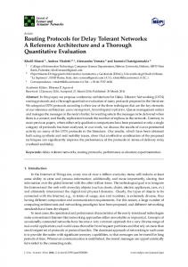
Fig. 1. Scenario 1: performance improvement of LSF Spraying over greedy Spray and Wait (SW) for different configurations; K =node’s transmission range, L = number of copies.
greedy LSF (cold) LSF (warm)
delivery ratio
L = 2 copies 0.489 0.63 (29%) 0.844 (72%) L = 4 copies 0.13 0.676 0.076 0.695 (3%) 0.117 0.841 (24%)
end-to-end delay protocol ( epidemic ) 1.59 1.44 (10%) 1.29 (22%) 1.41 1.355 (4%) 1.25 (13%)
are run normally in the first day, collecting encounter statistics, but without any traffic generated; traffic is generated and performance is measured only during the second day. Both the cold and warm versions are threshold-based (rule 1); however, in the warm version Uth is made large enough (58000 time units, which corresponds to more than one day’s time in the trace), to ensure that encounter statistics collected from day 1, carry over to day 2. “LSF (warm)” shows considerably higher improvement (72% higher delivery ratio and 22% better delays, for L = 2), demonstrating the power of utility-based replication, even in this small scenario. Finally, as the percentage of total nodes that get a copy increases (L = 4, i.e. around 20% of all nodes get a copy of a message), mistakes made by greedy replication are not as costly, and the improvement achieved by LSF is smaller. Summarizing, these trace-based results confirm the trends observed in the larger synthetic traces.
and uniformly distributed in the network, corresponding for example to base stations or static sensors. In Fig. 1 we depict the improvement in delivery delay, compared to that of greedy Spray and Wait (“SW”), when message replicas are handed over using LSF Spraying (rule 1 is used – threshold values Uth for this scenario were 500 − 1000 time units). As can be seen there, taking into account the age of last encounter when spraying the L copies can indeed improve performance. To further test the benefits of doing utility-based replication, we compare the performance of LSF spraying against greedy spraying and epidemic routing, in a trace-based scenario (Scenario 2). Specifically, we utilize traces from the DieselNet project (available at the CRAWDAD repository [54]), which record the encounters between buses of a public transportation network connecting various campuses in Amherst, in an area of approx. 150 square miles. We have performed simulations for a number of different traces from this repository, observing similar behaviors. These traces consist of only a small number of nodes (up to 24 buses), and the improvement achieved is naturally expected to be smaller than the one observed for the previous scenario of 100 nodes. Nevertheless, even in this small scenario the benefits of utility-based replication is clear. Table I shows results corresponding to trace #2182005. “Transmissions” shows the reduction in transmissions compared to epidemic. “Delivery Ratio” is the percentage of messages delivered. End-to-End Delay is the increase in delay compared to epidemic routing. We choose to compare our results against epidemic routing for a light traffic load, for which epidemic is close to optimal in terms of delay and delivery ratio. The values in the parentheses next to the delivery ratio and delay values for LSF correspond to the percentage improvement over greedy. “LSF (cold)” means that LSF is run directly on the trace for that day (Uth = 1000−5000 time units), without any previously collected history of encounters from past days. When 2 copies are used per message, you can see that LSF has a 29% higher delivery ratio, and a 10% smaller delivery delay, compared to the greedy algorithm. However, in a real life situation where the protocol will have been in operation for days or weeks, we expect past encounters from previous days to serve as valuable hints when choosing a relay. Unfortunately, the available traces are collected over a large period, and it is not clear if any of these and which ones correspond to consecutive days. Therefore, to “re-create” a scenario with consecutive days, we assume that the same trace is repeated for 2 consecutive days, and we examine the potential improvement by LSF on the second day (we denote this protocol as “LSF (warm)”)5 . In the “warm” version nodes
Here, we turn our attention to the MMF Spraying scheme. As we mentioned in Section III, MMF Spraying applies to scenarios where there exist multiple classes of nodes. Unfortunately, there do not exist such traces of hybrid networks, as most of them correspond to only one class of nodes (e.g. just vehicles [53], or just pedestrians [35], etc.). For this reason, for MSF and MMF we have only used synthetic simulations to evaluate their performance6 . In Fig. 2 we compare the delivery delay of MMF Spraying and Greedy Spraying, in the same scenario as Sec. IV-A (Scenario 1). We compare two levels of knowledge for the MMF scheme: (i) messages are given only to nodes of type “local” or type “roaming” but never to “static” or “community” (denoted as MMF1), and (ii) now a relay must also have {pl < 0.9 AND pr > 0.15} in addition to label “local” or “roaming” (MMF2). We show plots for both a very sparse network (< 8% of nodes are connected) and a denser one (“flakynet” – around 50% of nodes are connected). As can be seen by these plots, by choosing only nodes that actually have a chance to deliver a message we can get up to 2.5 − 3× reduction in delay in this scenario. Greedy spraying wastes many copies by handing them over to community and static nodes. Intuitively, the larger the amount of node heterogeneity the higher the expected improvement when using “smarter” copy replication. In this second scenario we assume only two types of nodes: (i) p% are “roaming” nodes that are useful as message relays and (ii) (1 − p)% are “community” nodes that are useless as message carriers, unless the destination lies inside their community (small probability). In
5 If a bus is used on different routes from one day to another one could presumably use the route and time information of the given bus rather than its physical ID, as the encounter related quantity of interest.
6 It would be of interest to try to combine some of the existing traces into a hybrid scenario. However, we defer looking into how and if such an endeavor would be successful for future work.
B. MMF Spraying
7
MSF Spraying (Delivery Ratio)
3 2.5 2 1.5 1 0.5 0
Protocol (# of copies)
Fig. 2. Scenario 1: performance improvement of MMF spraying over greedy Spray and Wait (SW), for two different connectivity scenarios (sparse and almost connected); L is the number of copies. MMF Spraying (Scenario 2) Delay (SW) / Delay (MMF)
5.5
K = 40, L = 16 K = 50, L = 10 K = 50, L = 16 K = 60, L = 16
5 4.5 4 3.5 3 2.5 2 1.5 1 0.4
0.3 0.2 0.1 0.05 percentage of mobile nodes (p)
Fig. 3. Scenario 2: performance improvement of MMF Spraying over greedy Spray and Wait, as a function of the percentage p of “useful” relay nodes; different configurations for K = nodes’ transmission range, and L = # of copies.
Fig. 3 we compare the performance of greedy Spray and Wait and MMF Spraying, which gives copies only to roaming nodes, as the percentage p of roaming nodes decreases. From this figure, it is evident that the smaller the percentage of useful (“roaming”) nodes, the higher the delay improvement by using smarter spraying. This is because greedy forwarding makes an increasing number of errors, wasting more and more copies ((1−p)L). On the other hand, we see that the achievable improvement peaks at a given value of p and starts becoming smaller again. At this point, the number of useful relays is so small (smaller than the number of copies) that the smarter Spraying scheme takes a very long time to find them. C. MSF Spraying In this last scenario we will examine the more practical scheme, MSF Spraying. Unlike the MMF scheme that uses preprocessed information (LABELs) to identify globaly useful relays, MSF tries to estimate this utility online by observing the type and number of encounters the node gets involved into. Fig. 4 compares the delivery delay for a scenario similar to that of Fig. 3, where only a percentage p of nodes are useful as message relays. It compares the performance of MSF to Greedy Spraying, as well as MMF spraying (which knows beforehand which are the useful nodes). The threshold-based MSF version is used (rule 1) with a sociability (Nth ) threshold chosen empirically between 5 and 107 . As can be seen there, both MSF and MMF improve the performance of Greedy spraying. What is more, MSF can approximate the performance of MMF without the fore-knowledge that the latter requires. (As a final note, although we do not have space to depict plots for the behavior of the running sociability estimates, we have observed that it manages to identify the “good” nodes after only a few windows.) have used L = 10 copies per message for all schemes, Tx range K = 30, the sliding window for MSF is 1000 time units, and α = 0.8.
MSF Spraying (Delivery Delay) 7000
Greedy
6000
MMF
5000
MSF
4000 3000 2000 1000 0
0.1 MMF1(L=10) MMF2(L=10) MMF1(L=16) MMF2(L=16)
7 We
1 0.9 0.8 0.7 0.6 0.5 0.4 0.3 0.2 0.1 0
deliv. delay(time units)
Delay (SW) / Delay (MMF)
sparse (8% connectivity) almost connected (52% connectivty)
delivery probability
MMF spraying (Scenario 1) 3.5
0.2
0.3
Ratio of "useful" nodes (p)
0.1 0.2 0.3 Ratio of "useful" nodes (p)
Fig. 4. Performance comparison of MSF, MMF, and greedy Spray and Wait, as a function of the percentage p of “useful” relay nodes.
V. P ROTOCOL T UNING Results in the previous section demonstrate that utility-based replication protocols can achieve significantly superior performance, when compared to greedy replication, in scenarios where node capabilities and behavior are heterogeneous. In this section, we discuss how to tune the main parameters of the proposed protocols in practice, in order to achieve such good performance; And, in addressing some practical issues, we also describe possible complementary mechanisms to the proposed protocols. A. Sliding Window for MSF Sociability Estimation The MSF replication algorithm is the most generic and practical, among the ones presented, as it can identify “social” nodes online. As was shown, it can achieve as good a performance as algorithms that know the “good” relays in advance (e.g. MMF). However,setting the sliding window parameters in MSF correctly (window duration T , and α) is necessary to achieve this. Let us define the stochastic sequence {Ni (n), n = 1, 2, . . . }, where Ni (n) is the number of unique node IDs encountered by node i during window tn : [(n − 1)T, nT ]. Whether or not the running sociability estimate Sˆn , based on past measurements in tn−1 , tn−2 , . . . , will be a useful predictor of future interactions (i.e. Ni (n+1), Ni (n+2), . . . ) depends on the amount of “structure” in the interaction and mobility patterns of the nodes involved, the window parameters, and the desired “horizon” for the prediction. Stationary Case: If the mobility process of all nodes in the network is stationary, then the sequence {Ni } will also be stationary. Thus, E[Ni (n)] = E[Ni ], ∀n and similarly E[Si (tn )] = E[Si (T )], ∀n.
The same holds for higher moments of the sequence (i.e. E[(Ni (n))k ] = E[(Ni )k ], ∀n, k). This implies that it is not important
during which time window ones looks at a node’s behavior. A node with a highly social past behavior will also have a social future behavior. An example of this could be if all nodes move according to the Random Direction model, but different nodes move with different average speeds and/or pause times. A node i with higher speed and shorter pauses than another node j , will meet on average more new nodes in the same amount of time than j , at any time scale8 . Since the statistics of the process do not change over time in the stationary case, what matters is choosing the value of α so that our sliding window estimator works efficiently. This depends on the variance σNi = E[(Ni )2 ] of the number of nodes encountered in each window. If the sociability variance of a node during different 8 We assume here that no encounters are missed. In reality, if a node moves very fast, it might not discover some contact opportunities which are short-lived, due to the workings of the neighbor discovery mechanism [35].
8
windows is high, it means that a small α value is needed to smoothen the estimate and ensure convergence. However, the smaller the α, the slower this convergence. One solution is for each node to maintain also the variance of the sampled sociability, in addition to the mean. This incurs little overhead and could be used to tune α according to the measured variance. Another solution would be to start with a relatively large α (aggressive) and keep increasing it until the oscillations of the running average from window to window, E[Sˆi (tn ) − Sˆi (tn−1 )] are smaller than some desirable threshold �. Cyclo-stationary (Periodic) Case: In real-life, people (and sometimes animals) often tend to have different mobility/interaction patterns during different times of the day. It has been frequently observed that real-life mobility exhibits such time-periodicity [58]. In this case, the statistics of the encounter sequence Ni might change as a function of time-of-day. This implies that, for some scenarios, the Ni (and, thus, Si ) could be modeled as a cyclo-stationary process. In these processes, if the sliding window T duration is smaller than the process’ cycle, then what happened in the previous time window cannot necessarily predict what will happen in the next. Yet, stationarity may also emerge here given a large enough time horizon for the prediction. If the duration of such a period is not prohibitive compared to the desired delivery delay9 , setting the sliding window T to this value would allow one to reliably predict future delivery probability in the next cycle. On the other hand, if finer granularity is needed for the prediction (i.e. targeted delays are much smaller than this period), one is forced to use a shorter sliding window. In this case, one could maintain multiple sociability values, corresponding to different time periods of the day (e.g. “morning”, or 2 − 4pm, etc.): then, each sample measured will affect only the time bin to which it corresponds, and inquiries about future delivery probability will take into account the sociability estimate corresponding to the time period(s) included in the horizon until the message in hand expires. Non-Stationary Case: In some cases, the mobility process of the nodes might be too complex to be modeled as a stationary or cyclo-stationary process. Nevertheless, mobility/interaction behavior in real life is never absolutely random. Even if the statistics (longterm behavior) of the process are changing, one would assume that these do so slowly. (Note that we do not here talk about the event of measuring different sociability values during different windows, something expected and predicted by the variance of the process, but rather the random process parameters changing.) In this case, the running average should still be able to follow and adapt to these changes, even so with a small lag that might just introduce a bit of error in the predicted delivery probability. B. Number of Copies Another important protocol parameter is the number of copies L to be used. This number has been calculated for Greedy Spraying in a homogeneous network, in order to achieve a desired transmissionvs-delay tradeoff [16]. The same procedure could be modified for the case of MMF spraying. The main idea is that, if there are M total nodes and MMF uses only p percent of them based on their labels, then this is equivalent to a network of pM nodes (some care is needed though, regarding the effect of the other (1 − p)M nodes in the minimum/optimal delay [16]). 9 Given the delay-tolerant nature of the targeted services (e.g. advertisements, email, message boards) and some of the targeted environments (e.g. developing countries, remote villages, etc.) it is not difficult to imagine that, for some users, delays as large as one day or more (i.e. equal to the daily process’ cycle) could be acceptable.
In the case of MSF Spraying, a different approach could be taken, as described by Lemma 5.1. Lemma 5.1: Assume there are M total nodes in a network moving independently of each other, and messages have a TTL value of Tmax . Let further each node use the MSF algorithm (rule 1) with sliding window T = Tmax , and threshold sociability value th Sth = TNmax . If the desired delivery probability for each message is Rmin , then the number of copies per message Lmin and sociability threshold must satisfy 1− 1−
Nth N
�L
min
≥ Rmin ,
(3)
where N is the total number of nodes. The above lemma can be derived by setting the sliding window duration T equal to the TTL value (Tmax ). Then, the sociability th . Nth becomes an estimate of the threshold would become TNmax unique number of nodes encountered within the message’s lifetime and thus of the delivery probability NNth of one relay, assuming that relays encounter other nodes in the network independently. If Lmin relays are used in total, the probability of delivery before the TTL expires is thus 1−(1− NNth )Lmin . Although this might not be realistic in practice, it could serve to either find a minimum Sth given Lmin or Lmin given Sth , if the sliding window is T = Tmax . An interesting question arises when one considers how to scale this value for a smaller time window. For example, consider how the parameters used for MSF in the case of Fig. 4 fit this equation. The main problem in this case is that the sliding window there is T = 1000 (with Nth = 5 − 10), while Tmax = 10000; thus we only have an estimate 1 of a packet’s of the average number of nodes encountered during 10 lifetime. If N1000 is the average sociability when the window is T = 1000, what can we say about N10000 ? Linear scaling (i.e. Nth = 50−100) gives too optimistic results (0.99 delivery ratio). The correct value of Nth corresponding to a sliding window of Tmax = 10000, to achieve Rmin ≥ 0.9 (as in Fig.4) seems to be around Nth = 25. We believe prediction methods like the one used in [16] could provide the answer to this scaling question, but we defer this for future work. In general, the joint problem of choosing both the number of copies and the copy bearers optimally is difficult. We assume here that either the number of copies is set by the application (e.g. credits per message) or the protocol is fixed and the network parameters known. Nevertheless, we next discuss a methodology that could potentially address the joint optimization problem. C. Copy Allocation as Portfolio Management: Whether the nodes’ mobility process is stationary or not, maintaining higher moments of a node’s past sociability can allow a node to make more “educated” decisions when allocating message copies. ˆSi }, For example, assume that each node maintains a tuple {Sˆi , σ that is, estimates of the node’s average sociability and its variance, respectively. Let, for example, a node carrying an extra copy of a ˆ Si � σ ˆ Sj . message encounter nodes i and j . Let further Sˆi > Sˆj but σ This means that, although node i is more sociable in general than j it is also much more “risky”: its future behavior cannot be reliably predicted. Also, whether i or j should get the extra copy, should also depend on who the other relays having received a copy are. A list of the relays that have received a copy can be maintained, with a predicted delivery profile (expected delay and variance) based on their joint characteristics. Then, every new copy forwarded should aim to improve this profile. For example, if we know that a number of “consistently” social nodes (i.e. good sociability with small variance)
9
already have a copy, it might be worthwhile to risk giving a copy to i, which might have some chance of delivering the copy faster than other relays, as opposed to using yet another “average” relay. This results into more complex, but also more powerful forwarding decisions, as opposed to simply comparing average values. Although we have described this procedure in the context of MSF, it is important to note that it could be also applied to other utility-based replication variants, e.g. LSF. In the case of LSF, a ˆTid } with estimates of the average and variance of the tuple {Tˆid , σ intermeeting time would be maintained. In general, the problem of allocating copies to nodes with different expected “return” (e.g. delivery delay) and different “risk” (e.g. variance of predicted delivery delay), is, in some aspects, equivalent to optimal asset allocation and portfolio theory in finance [59]. An interesting effort uses ideas from modern portfolio theory to address some reliability issues [38]. We intend to look more into this issue in future work. D. Avoiding Node Overloading If message replicas are handed over to a few good nodes, then these nodes might absorb a disproportionate amount of workload compared to the average node. Accepting a copy implies a particular overhead for a node in terms of buffer space, battery power, and bandwidth consumption. Nevertheless, in many scenarios of interest node overloading is not a concern. For example, in situations where some nodes (e.g. buses with no energy constrains [53]) have considerably more resources than the average node (e.g. a pedestrian carrying a PDA), it is desirable to direct more traffic to the over-provisioned nodes. Furthermore, if overusing a particular node resource is a concern, one could incorporate the usage of this particular resource into a (hybrid) utility function that aims at optimizing a combination of different goals. For example: Remaining battery level: a node may use a hybrid utility function Uˆ = f (Uorig , power), where Uorig captures the probability of message delivery (i.e. Uorig = {U LSF , U MMF , U MSF }) and power is the remaining battery level (taking values in [0, 1]). Then the forwarding rule could be defined as: ˆ = Uorig ; • if power > powermin then U ˆ = 0. • if power < powermin then U This policy sets a “cutoff” (powermin ) preventing nodes to serve as relays when their remaining lifetime is below a certain level. Another policy could weigh the advertised utility by the remaining power: ˆ = power × Uorig U 1 ˆ =1− U (Uorig )power
(linearly) (non − linearly).
A similar mechanism could be employed to prevent a node from serving as a relay if its buffer occupancy drops below a threshold. Thus, under light loads the protocol operates with routing efficiency in mind, while at high loads it makes load-balancing a factor. E. Security Considerations: Counterfeiting Utility Allowing “gravitational points” that attract a high proportion of the network load can also become a security “loophole”. Ideally, the node that forwards the copy(ies) trusts the next hop to be stating its true, measured utility. Thus, if a malicious node decides to advertise a very high (fake) utility value, it can easily absorb a large number of messages. It could then just drop them (DoS) or try to read/decode them (compromise privacy). The proposal of security solutions for delay-tolerant networking is beyond the scope of this paper. We should point out that it is an
area of active research. For instance, some security-related issues arising from intermittent connectivity have been partly addressed in [60]. Reputation mechanisms based on monitoring neighboring transmission are revisited in [61], since such monitoring is difficult in sparse networks. The studies reported in [21, 62] show that the very nature of epidemic replication makes it quite resilient to many types of attacks. Finally, it has been shown that mobility itself could facilitate the establishment of a robust trust system on the fly [63]. VI. P ERFORMANCE A NALYSIS OF E NCOUNTER - BASED ROUTING IN H ETEROGENEOUS N ETWORKS Having concentrated in the previous sections on the protocol performance and tuning, in this last section, we embark on developing appropriate theoretical models for encounter-based message dissemination in heterogeneous networks. These models not only aim to help us analyze the performance of the routing schemes presented, but can also serve as the foundation to analyze various other encounter-based processes (e.g. wireless virus spread [64]) in networks consisting of mixed populations of nodes. Our theoretical framework is a based on an appropriate fluid model formulation for epidemic routing [19], in a heterogeneous setting. The basic concepts and terminology are borrowed from the field of Epidemiology and Mathematical Biology [26]. Nodes having already received a copy (we call these nodes “Infected”, I ) may forward an additional copy to a node not having yet received one (we call this nodes “Susceptible”, S ). We are then usually interested in the expected time until a given node (e.g. destination) gets infected (i.e. receives the message) or the probability of this occurrence (delivery ratio). A fluid model can then be formulated that captures the rate of message propagation (“infection”) among nodes and can be used to calculate the above quantities. Our model extends the fluid model formulation of [27], which was proposed for homogeneous networks with a single class of nodes. Although fluid models are only a deterministic approximation of the stochastic spreading of messages using epidemic routing, they produce accurate results for moderate to high numbers of networks nodes [27]. We have chosen to start by modeling epidemic routing first for the following reasons: (i) epidemic routing [19] is the first, and among the most generic opportunistic routing protocols proposed with many variants having followed (e.g. Prophet [20], SLEF [62], etc); (ii) its delay is minimum under ideal conditions (little or no contention for shared resources like bandwidth and buffer space), and thus can serve as an optimality baseline; (iii) we will use it to describe a version of controlled replication (greedy and utility-based), that is equivalent to the one originally presented [22], but is more amenable to our fluid model based analysis. Having developed this basic model for epidemic routing, we then use it to quantify the performance of Greedy Replication when node mobility is heterogenous (the homogeneous case is treated in [17, 22]). Finally, we analyze how good a delay we can achieve, as compared to the optimal case, by using Smart Replication algorithms like MSF or MMF. Before we proceed, it is important to define node heterogeneity in a rigorous manner. Our model for a heterogeneous network consists of multiple classes of nodes (k total), with different intra- and interclass meeting characteristics. The reason for this choice is two-fold: (i) this setting can successfully capture two scenarios of high interest, one, scenarios where nodes are naturally separated into communities or groups with high intra-group meeting rate (e.g. same department, affiliation, family), and two, scenarios where some subsets/classes of nodes have different characteristics or capabilities than others (e.g. vehicles, pedestrians, base stations, etc.); (ii) this multi-population
10
TABLE II N OTATION N M Mi βij EMij = Ii (t)
size of network area total number of nodes number of nodes of class i mixing rate between nodes of classes i and j exp. meet time between nodes of class i and j
1 βij
Dprotocol P (t)
infected nodes of class i at time t delivery delay of protocol “protocol” complementary cumulative distribution function of random variable X(t): P (t) = P rob(X(t) > t)
model is more amenable to fluid model analysis; it has also been used often in epidemiology from which we might be able to borrow some results or formalisms. In the remainder of this section we will assume the following: (a.) There are M nodes in total, each moving according to some stochastic mobility model in a finite area. This mobility is neither known in advance [2] nor enforced [29]. (b.) Each of the M nodes belongs to a particular mobility class i, among k possible ones. Nodes in different classes may move according to different mobility models (e.g. some nodes perform random walks, while others perform random direction mobility) or simply have different mobility parameters (e.g. all nodes perform random waypoint mobility, but nodes in one class have high average speed and small pause times). � The total number of nodes in class i is denoted as Mi with ki=1 Mi = M . (c.) Let a node i belong to mobility class i ∈ [1, k] and another node j belong to mobility class j ∈ [1, k]. Further, let the two nodes start from their stationary distributions at time 0. The meeting time (Mij ) between them is defined as the time it takes to first come within range of each other, that is Mij = min{t : t �Xi (t) − Xj (t)� ≤ K}, where K is the maximum transmission range, and Xi (t) is the position of node i at time t. (d.) We define the meeting or “mixing” rate between the two classes i and j , βij as the inverse of the expected meeting time for these 1 . The mixing rate is a measure of how often classes: βij = EM ij a node of one class meets a given other node of another (or the same) class. We will assume that all meeting times Mij , i, j ∈ [1, k] are approximately exponentially distributed (or have an exponential tail [48]) with expected value EMij = β1ij . It has been shown that a number of popular mobility models have such exponential tails (e.g. Random Walk, Random Waypoint, Random Direction, Community-based Mobility [41, 56]). (e.) Ii (t) denotes the number of nodes of type i that have already been infected (i.e. have received a copy) at time t.
“buffer cleaning” policy10 , the spreading of this message is given by the solution of the following system of rate equations:
� dIi (t) Ij (t)βji (t), ∀i ∈ [1, k] = (Mi − Ii (t)) dt k
Is (0) = 1, Ij (0) = 0, ∀j �= s.
Proof: A fluid model approximation for a single class of nodes has been formulated and justified in [27]. Here, we extend this formulation into multiple classes, using similar arguments and assumptions about scaling as [27]. Let us assume that there are Ii (t) nodes of class i that have received a copy of the message (i.e. are “infected”) at time t. The number of susceptible nodes of class i are Mi − Ii (t). If there are also Ij (t) nodes infected from class j and individual nodes of classes i and j encounter each other (i.e. mix) with rate βij , then the probability of a new node of class i getting infected by a class j node at the next time instant Δt → dt is Ii (t + dt) − Ii (t) = βij (Mi − Ii (t))Ij (t)dt.
Taking into account also all other classes j ∈ [1, k] of nodes that can (independently) infect nodes of class i gives us the system of Eq.(4). Initial conditions simply state that only a node from class s is infected at first. The next theorem derives the complementary cumulative probability distribution function (CCDF) of the delay until a message is delivered to a randomly chosen destination. The CCDF completely describes the delivery delay for epidemic routing (expected value and higher moments). Theorem 6.1: Let’s assume that the destination for the message propagated in Lemma 6.1 belongs to class “d”. Let further, the CCDF (Complementary Cumulative Distribution Function) of the delay until the destination receives the message be denoted as P = P (Depid > t). Then, P is given by solving the following equation:
� dP (t) βid Ii (t), = −P (t) dt
In this section, we start by modeling the performance of the Epidemic Routing protocol [19] in heterogenous networks. A similar formulation for multiple populations can be found in the context of Mathematical Biology, yet with different quantities of interest in mind (e.g. epidemic threshold) [45]. Lemma 6.1: Let’s assume that there are k classes of nodes, and that one message from a node in a class s ∈ [1, k] originates at time t = 0. If this message is propagated using epidemic routing and no
(5)
i
where Ii (t) are given by Lemma 6.1. Proof: Let us calculate the probability P (Depid > t + dt). It is easy to see that P (Depid > t + dt) = P (Depid > t) × (1 − P rob(t ≤ Depid ≤ t + dt)).
Since meetings between nodes are approximated by a Poisson process, the probability of the destination being found at any instant of duration dt is equal to the aggregate meeting � rate of infected nodes with the destination at time t times dt: i Ii (t)βid dt. Thus
�
P (t + dt) ⇒
A. Epidemic Routing
(4)
j=1
P (t + dt) − P (t) dt
= =
P (t) 1 − −P (t)
�
�
�
Ii (t)βid dt
i
Ii (t)βid .
i
Based on the above density function, the expected delay for epidemic routing in this multi-class population follows easily from elementary probability. Corollary 6.1: The expected delay of epidemic �routing in a network of k node populations is given by EDopt = P (t)dt. 10 In [17], it is suggested that “anti-packets” are propagated back to infected nodes after the message reaches its destination, in order to release some buffer space and avoid further infection. These nodes would then be considered ”Recovered” (R), and an SIR model would be more appropriate. Without loss of generality, here, we decide to treat the simpler case of no anti-packets (i.e. “No-Immune” version in the paper).
11
50
80
I1(t)
60
M1=50, M2=50
Infected Nodes
100
40
I2(t) I1(t)
30
40
20
I2(t)
20
2-class Population 600
delivery delay
M1=100, M2=20
Infected Nodes
10 0.05
0.1
0.15
0.2
0.25
Time 0.02 0.04 0.06 0.08 0.1 0.12 0.14
500
sim
400
theory
300 200 100
Time
0 0.1
0.2
0.3
0.4
0.5
ratio of mobile nodes (p)
Fig. 5. Number of infected nodes in class 1 (I1 - static nodes) and class 2 (I2 mobile nodes), as a function of time. We have normalized time and mixing rates such that β11 = 0, β12 = 1, β22 = 2. CCDF : P H D > tL 1
M1 = 100, M2 = 20 M1 = 50, M2 = 50
0.8
Def. 6.1. This one is more amenable to a fluid model analysis, and has equivalent performance to the original scheme, on average. Definition 6.1 (Time-Bound Spray & Wait): Let’s assume a message gets created � at time Tstart . Let further Tspray be such that I(Tspray ) = i Ii (Tspray ) = L, where Ii (t) are given by Lemma 6.1. Then,
0.6 0.4 0.2
0.05
0.1
0.15
0.2
0.25
t
Fig. 6. CCDF of the delivery delay, for the two scenarios of Fig. 5. Destination is chosen uniformly in class 1.
Two mobility classes (k = 2): To get some insight into the above formulation, we will look in more detail into the special case of only 2 classes of nodes, as in Section III-A. Specifically, we will assume that the network comprises: (class 1) a fraction of nodes 1 − p that move more slowly and rarely than nodes in the second class (b22 � b11 ) or are static (b11 = 0), (class 2) a fraction of nodes p that move frequently and/or fast around the network (e.g. vehicles). In this case the system of ODEs of Lemma 6.1 becomes: dI1 (t) = (M1 − I1 (t))(I1 (t)β11 + I2 (t)β12 ) dt dI2 (t) = (M2 − I2 (t))(I1 (t)β12 + I2 (t)β22 ) dt I1 (0) = c1 , I2 (0) = c2
Fig. 7. Comparison of analytical and simulation results for the expected delay of epidemic routing; M = 300 total nodes in a 1000 × 1000 network with, and K = 30; p of the nodes move according to the Random Direction model, while 1 − p are static.
(6) (7) (8)
In Fig. 5 we depict I1 (t), I2 (t), the total number of infected nodes of each class as a function of time, for different values for M1 , M2 , and in Fig. 6 we depict the respective cumulative probability density functions. It is easy to observe from these figures that, when there are more “fast” nodes in the network (class 2) infection is faster, and delivery delay smaller. Finally, in Fig. 7 we compare simulation results for the delay of epidemic routing against analytical values calculated according to Corollary 6.1, again for a scenario of 2 populations of nodes, as a function of the ratio between nodes of the two classes. We observe that theoretical and simulation results are closely matched, which confirm the accuracy of our fluid model. B. Controlled Replication (Spraying) Here, we will turn our attention into analyzing the delay of Controlled Replication, both greedy and utility-based. The delay of greedy replication (Spray and Wait) has been analyzed using probability theory and Markov Chains in [16, 17, 22], for homogeneous node scenarios. To calculate the delay in heterogenous networks, we will use again fluid models, as in the previous section, due to their power to model population mixing problems. However, instead of using the scheme described in Def. 3.1, we will use the variant of
•
(spray phase) all nodes (source and relays) perform epidemic forwarding (i.e. give a copy to every new node encountered) until time Tstart + Tspray ; • (wait phase) after time Tstart + Tspray , any node that has received a message copy, may only give a new copy to the message destination. The above scheme emulates greedy, tree-based replication with L copies (see Section III-A). 1) Greedy Replication: Theorem 6.2: Let’s assume that there are k classes of nodes in a � network with M total nodes (M = ki=1 Mi ). Let further a message originate at time t = 0 from a node in a class s ∈ [1, k] and destined to a node of class d ∈ [1, k]. Let further this message be routed using the time-bound Spray & Wait protocol of Definition 6.1. Then, the expected delivery delay of the message, EDsw , is upper bounded by EDsw ≤ Tspray +
�
k 1 M − i=1 Ii (Tspray ) , � k M i=1 βid �Ii (Tspray )�
(9)
where Ii (Tspray ) are given by Lemma 6.1. Proof: Tspray is the time during which message copies are distributed to relays (using epidemic spreading as described in Defin� ition 6.1). During this time ki=1 Ii (Tspray ) copies are given in total, where Ii (t), i ∈ [1, k] are given by Eq.(4). Since source-destination pairs are chosen uniformly among all nodes, the probability that the destination has not been found during the copy distribution phase M− k i=1 Ii (Tspray ) . In that case, each of is equal to P (wait) = M the L nodes will hold on to its message copy until it encounters the destination itself (or TTL expires). Let us denote this additional time as Twait , and let at the end of Tspray exist �Ii (Tspray )� relays of class i (since no fractions of nodes can exist). If we assume that each one of them meets the destination independently, and the individual meeting times are exponential with average β1id for class i, then
�
Twait =
�k
1
i=1 �Ii (Tspray )�βid
.
Putting it altogether EDsw ≤ Tspray +
M−
�k
Ii (Tspray ) �k β �I1 (T )� . M spray i=1 id i
i=1
12
The reason why the above is an upper bound is that we always count the whole spraying delay, Tspray , even if the destination was actually found before the end of the replication timer. Nonetheless, if L � M (the case we are most interested in, since we want to drastically reduce the number of nodes that are burdened with a copy), then the above bound becomes tight, similar to the singlepopulation case [22]. 2) Utility-based Replication: Next, we will look into the delay of Utility-based Replication that allows only nodes in particular classes to act as relays. Although this is typically the MMF routing protocol, it can also model MSF routing with appropriately chosen thresholds. We start with a special case that is easier to handle, where only one class of nodes can act as relays. We can adapt the results of [16] to calculate the delay for this case, without resorting to fluid models. We use the fluid model next to address the general case. Lemma 6.2: Let’s assume that a message, from a node in a class s ∈ [1, k] to a node of class d ∈ [1, k], is routed with MMF spraying using only nodes of some class r ∈ [1, k]. Further, let EDMMF (L + 1) be the expected delay of the scheme, when L + 1 copies are used. Finally, let ED(i) be the expected remaining delay after i message copies have been spread. Then, ED(1) ≈ EDMMF (L + 1), where ED(1) is calculated by the following system of recursive equations: �
ED(i)
=
ETnext (i) + Pnext (i)ED(i + 1), i ∈ 1,
ED(i)
=
ETnext (i) + Pnext (i)[
ED(L + 1)
=
2i − L ED(i) + i � L L−i ED(i + 1)], i ∈ + 1, L − 1 ; i 2 1 , Lβrd + βsd
L ; 2
In a manner similar to Theorem 4.2 of [16] we can show that a useful approximation is Xi = i, i ∈ [1, L/2] and Xi = L − i, i ∈ [L/2 + 1, L − 1]. Finally, if all L copies have been distributed (1 at source and L at nodes of class r), and the destination has not been found yet, then the remaining time is easily found to be ED(L + 1) = Lβrd1+βsd . Theorem 6.3 addresses the general case where utility-based spraying may use more than one classes of nodes as relays. Its proof follows a similar methodology as Lemma 6.1. Theorem 6.3: Let a message be routed using the time-bound Spray & Wait protocol of Definition 6.1. However, assume further that only a subset of classes R can act as relays, R ⊂ [1, k] (i.e. MMF/MSF spraying). Then, the expected delivery delay of the message EDMMF is upper bounded by EDMMF ≤ Tspray +
�
k 1 M − i=1 Ii (Tspray ) � , M i∈R �Ii (Tspray )�βid
where Ii (Tspray ) are given by Lemma 6.1. Proof: The proof goes along the same lines as that of Theorem. 6.2, with the difference that the nodes of classes � who cannot / R) are ignored. Also, note that L = i∈R Ii (t), the act as relays (∈ total number of copies distributed after Tspray , will be smaller here than the value of Theorem. 6.2, everything else equal. To make sure that the average number of copies distributed for MMF spraying is equal, on average, as in the greedy replication case, we need to set Tspray (M M F ) such that: Tspray (M M F ) = arg min{ t
Pnext (i)
= =
�
�
1
(i − 1) (Mr − i + 1)) βrr +
βsr i−1
�
�
+ βrd + βsd
(Mr − i + 1)(βrr (i − 1) + βsr ) . (Mr − i)(βrr (i − 1) + βsr ) + (i − 1)βrd + βsd
,
Proof: This proof follows a similar methodology as that of Theorem 4.2 in [16]. Let us look into the case, when there are i nodes (i < L) that have one or more copies. Since the source always has at least one copy, this would imply that there are i − 1 relays of class r and one of class s. Further, let’s assume that, among the i nodes with copies, Xi of them have more than one copy (“active”), and are allowed thus to forward copies further to other relays. Since all hitting times are independent and exponentially distributed, nodes with a message copy (i total) encounter: (i) any of the nodes of class r without a copy (Mr − i) with rate (i − 1)(Mr − i)βrr + (Mr − i)βsr or (ii) the destination itself with rate iβrd +βsd . This is the time until the next encounter of interest occurs (either a candidate relay or the destination), and we shall denote it as ETnext (i). Now, if the node encountered is the destination, the message gets delivered. Otherwise (Mr −i+1)(βrr (i−1)+βsr ) (with probability Pnext (i) = (Mr −i)(β ) rr (i−1)+βsr )+(i−1)βrd +βsd the algorithm continues, performing one of the following: a) with probability Xi i it is one of the “active” nodes that encountered this other node, and therefore hands it over half its copies; i + 1 nodes have copies now, and an expected time ED(i + 1) remains until i delivery; b) with probability i−X it was one of the other nodes i carrying a message copy that encountered a new node. Since these relays only forward their message copy to its destination, nothing happens, and the remaining time is still ED(i). Putting it altogether � ED(i) = ETnext (i) + Pnext (i)
�
i − Xi Xi ED(i) + ED(i + 1) . i i
�
Ii (t) = L} ≥
i∈R
where ETnext (i)
(10)
k �
Tspray (greedy) = arg min{ t
Ii (t) = L}.
i=1
This implies that the first component in the right-hand side of Eq.(10), Tspray , will be larger in the MMF case than in the greedy case (Eq. 9). The reason is that, in the greedy case, after L nodes with no copy are encountered, the spraying phase always ends; in the utility-based case, the first L nodes do not necessarily become relays (if they don’t have high enough utilities). Thus, the spraying phase continues and finishes only after enough nodes have been met (say L� ≥ L), such that L of them had a high enough utility to receive a copy. For the same reason, the probability that the destination is found during the “spraying” phase for MMF is Putil (wait) = � L� M ; if one of the L nodes encountered is the destination, the message gets delivered. Since, in the greedy case, this probability L , and L� ≥ L, it follows that the probability is Pgreedy (wait) = M of finding the destination in the spraying phase, is higher for MMF. In fact, if the subset of candidate relays (classes in R) becomes sufficiently narrow (total number of nodes in classes in R is smaller than L), then the destination is always found during the spraying phase. The following Lemma and its Corollary 6.2 compare the performance of greedy replication and utility-based replication in multiplepopulation scenarios. Lemma 6.3: The expected remaining delay (“wait phase delay”) after all copies, let L, have been distributed is always smaller in the case of MMF than in the case of greedy replication. Proof: Let’s assume that Tspray (M M F ) and Tspray (grd) are such that L copies are distributed on average for both MMF and greedy replication. Then,
13
� (1)
�
(2)
�
(3)
�
IiM M F (t)βid
i∈R
=
Iigrd (t)βid +
i∈R
≥
Iigrd (t)βid + min{βid } i∈R
Iigrd (t)βid
�
(5)
k �
≥
Iigrd (t)βid +
IiM M F (t) − Iigrd (t)
�
Ijgrd (t)
ˆ j∈R
Ijgrd (t)βjd
ˆ j∈R
i∈R
=
i∈R
�
�� i∈R
+ min{βid }
i∈R
(4)
IiM M F (t) − Iigrd (t) βid
i∈R
i∈R
=
��
Ijgrd (t)βjd .
j=1
�
Step (1) is simply adding and subtracting i∈R Iigrd (t)βid . Step (2) follows by replacing each βid ,i ∈ R with the minimum value among them. Since the number of copies spread for both the the utility-based cases is equal to L, it holds that �greedy � and grd I (t) = IiMMF (t) − Iigrd (t) . This simply says that the ˆ j j∈R rest of copies, which in the MMF case are given to some nodes of ˆ ) in greedy classes in R, are given to nodes in classes outside R (R replication. This gives step (3). Step (4) follows from the fact that nodes in any class in R mix faster with the destination that nodes / R. Step (5) is in any class outside R. Thus min{βid } ≥ βjd , ∀j ∈ i∈R simply merging the two sums. Consequently, 1
�
i∈R �Ii (Tspray (M M F ))�βid
≤
�k
1
i=1 �Ii (Tspray (grd))�βid
Corollary 6.2: Let s and d denote the node class of the source and / R, where the destination of a message, respectively, and let s, d ∈ R is the set of classes that can act as relays in the MMF replication βkl algorithm. Finally, let Lβ > 1, ∀i, j, k ∈ R, and ∀l ∈ R. Then, the ij expected delivery delay of the M M F algorithm EDMMF is always smaller than the expected delay of greedy replication EDgrd . Proof: This can be derived using some calculations from Lemma 6.3 and Theorem 6.3. Lemma 6.3 and Corollary 6.2 essentially say that, if data sources and sinks do not generally mix but rely on a set of “special”, mobile nodes to carry traffic around, then utility-based replication is always faster than greedy replication. This would be the case for example when nodes are either static (sensors) or slowly moving (pedestrian) while routers are vehicles like buses [53]. As a final note, we have also compared simulation and analytical results (bounds) for greedy and utility-based replication for heterogenous networks consisting of 2 populations of nodes, as in the epidemic routing case (Section VI-A). We have observed that respective results present a similarly good match, so we choose to not include the plots due to space limitations. VII. C ONCLUSION In this work, we have looked into the issue of efficient mobilityassisted or opportunistic routing for networks comprising heterogeneous node populations. We have explored the issue of allocating a fixed budget of message replicas among a number of candidate relays with different capabilities and mobility patterns. To this end, we have proposed a number of simple heuristics that try to capture
how probable it is for a given relay to encounter the destination in the near future. Using both theory and simulations, we show that choosing the relays carefully rather than picking the first few relays encountered [16–18], can significantly improve performance in heterogeneous scenarios. Possible directions for future work include exploring the design of more sophisticated or hybrid heuristics, as well as addressing the issue of optimally solving the joint number-of-copies/copy-allocation problem. Yet, we believe that this work clearly shows that utilitybased replication presents a desirable and often necessary routing mechanism, when the number of total transmissions needs to be controlled, while at the same time not all nodes in the network are equally useful for routing. Finally, using utility-based replication rather than greedy replication during the initial distribution phase of message replicas could also have an improvement on the performance of schemes that allow multi-hop forwarding [16]. R EFERENCES [1] A. Seth, D. Kroeker, M. Zaharia, S. Guo, and S. Keshav, “Low-cost communication for rural internet kiosks using mechanical backhaul,” in Proceedings of ACM MobiCom, 2006. [2] S. Jain, K. Fall, and R. Patra, “Routing in a delay tolerant network,” in Proceedings of ACM SIGCOMM, Aug. 2004. [3] A. Pentland, R. Fletcher, and A. Hasson, “DakNet: Rethinking connectivity in developing nations,” IEEE Computer, vol. 37, no. 1, pp. 78–83, 2004. [4] P. Basu and T. Little, “Networked parking spaces: architecture and applications,” in Proceedings of IEEE VTC, 2002. [5] M. Papadopouli and H. Schulzrinne, “Seven degrees of separation in mobile ad hoc networks,” in Proceedings of IEEE GLOBECOM, 2000. [6] M. Motani, V. Srinivasan, and P. S. Nuggehalli, “PeopleNet: engineering a wireless virtual social network,” in Proceedings of ACM MobiCom, 2005. [7] P. Hui, A. Chaintreau, J. Scott, R. Gass, J. Crowcroft, and C. Diot, “Pocket switched networks and human mobility in conference environments,” in Proceedings of ACM SIGCOMM workshop on Delay Tolerant Networking (WDTN), 2005. [8] “Disruption tolerant networking,” http://www.darpa.mil/ato/solicit/DTN/. [9] J. Heidemann, W. Ye, J. Wills, A. Syed, and Y. Li, “Research challenges and applications for underwater sensor networking,” in Proceedings of IEEE WCNC, 2006. [10] “Delay tolerant networking research group,” http://www.dtnrg.org. [11] E. Brewer, M. Demmer, B. Du, M. Ho, M. Kam, S. Nedevschi, J. Pal, R. Patra, S. Surana, S. Surana, and K. Fall, “The case of technology for developing regions,” IEEE Computer, vol. 38, no. 6, pp. 25–38, 2005. [12] B. Du, M. Demmer, and E. Brewer, “Analysis of WWW traffic in cambodia and ghana,” in Proceedings of WWW’06 conference, 2006. [13] P. Juang, H. Oki, Y. Wang, M. Martonosi, L. S. Peh, and D. Rubenstein, “Energy-efficient computing for wildlife tracking: design tradeoffs and early experiences with zebranet,” in Proceedings of ACM ASPLOS, 2002. [14] E. P. Jones and P. A. Ward, “Routing strategies for delay-tolerant networks,” available at http://ccng.uwaterloo.ca/ pasward/Publications/. [15] T. Spyropoulos, K. Psounis, and C. S. Raghavendra, “Efficient routing in intermittently connected mobile networks: the single-copy case,” IEEE/ACM Trans. Netw., vol. 16, no. 1, pp. 63–76, 2008. [16] ——, “Efficient routing in intermittently connected mobile networks: the multiple-copy case,” IEEE/ACM Trans. Netw., vol. 16, no. 1, pp. 77–90, 2008. [17] T. Small and Z. Haas, “Resource and performance tradeoffs in delay-tolerant wireless networks,” in Proceedings of ACM SIGCOMM workshop on Delay Tolerant Networking (WDTN), 2005. [18] G. Neglia and X. Zhang, “Optimal delay-power tradeoff in sparse delay tolerant networks: A preliminary study,” in Proceedings of ACM SIGCOMM workshop on Challenged Networks (CHANTS’06), 2006. [19] A. Vahdat and D. Becker, “Epidemic routing for partially connected ad hoc networks,” Duke University, Tech. Rep. CS-200006, 2000. [20] A. Lindgren, A. Doria, and O. Schelen, “Probabilistic routing in intermittently connected networks,” SIGMOBILE Mobile Computing and Communication Review, vol. 7, no. 3, 2003. [21] J. Burgess, G. Bissias, M. Corner, and B. Levine, “Surviving attacks on disruption-tolerant networks without authentication,” in Proceedings of ACM MobiHoc, 2007.
14
[22] T. Spyropoulos, K. Psounis, and C. S. Raghavendra, “Spray and Wait: Efficient routing in intermittently connected mobile networks,” in Proceedings of ACM SIGCOMM workshop on Delay Tolerant Networking (WDTN), 2005. [23] H. Dubois-Ferriere, M. Grossglauser, and M. Vetterli, “Age matters: efficient route discovery in mobile ad hoc networks using encounter ages,” in Proceedings of ACM MobiHoc, 2003. [24] S. Zhong, J. Chen, and Y. R. Yang, “Sprite: A simple, cheat-proof, credit-based system for mobile ad-hoc networks,” in Proceedings of IEEE INFOCOM, 2003. [25] T. Spyropoulos, T. Turletti, and K. Obraczka, “Utility-based message replication for intermittently connected heterogeneous wireless networks,” in Proceedings of IEEE WoWMoM Workshop on Autonomic and Opportunistic Communications (AOC), 2007. [26] D. J. Daley and J. Gani, Epidemic Modelling: An Introduction. Cambridge University Press, 2001. [27] X. Zhang, G. Neglia, J. Kurose, and D. Towsley, “Performance modeling of epidemic routing,” in Proceedings of IFIP Networking, 2006. [28] V. Lenders, G. Karlsson, and M. May, “Wireless ad hoc podcasting,” in Proceedings of IEEE SECON, 2007. [29] W. Zhao, M. Ammar, and E. Zegura, “A message ferrying approach for data delivery in sparse mobile ad hoc networks,” in Proceedings of ACM MobiHoc, 2004. [30] M. S. Alexander Hall, Steffen Hippler, “Multicommodity flows over time: Efficient algorithms and complexity,” in Proceedings of ICALP, 2003. [31] B. Hoppe and E. Tardos, “The quickest transshipment problem,” in Proceedings of SODA, 1995. [32] E. P. C. Jones, L. Li, and P. A. S. Ward, “Practical routing in delay-tolerant networks,” in Proceedings of ACM SIGCOMM workshop on Delay Tolerant Networking (WDTN), 2005. [33] N. Sarafijanovic-Djukic, M. Piorkowski, and M. Grossglauser, “Island hopping: Efficient mobility-assisted forwarding in partitioned networks,” in Proceedings of IEEE SECON, 2006. [34] J. Ott, D. Kutscher, and C. Dwertmann, “Integrating DTN and MANET routing,” in Proceedings of the 2006 SIGCOMM workshop on Challenged networks (CHANTS), 2006. [35] A. Chaintreau, P. Hui, J. Crowcroft, C. Diot, R. Gass, and J. Scott, “Impact of human mobility on the design of opportunistic forwarding algorithms,” in Proceedings of IEEE INFOCOM, 2006. [36] J. Burgess, B. Gallagher, D. Jensen, and B. N. Levine, “MaxProp: Routing for Vehicle-Based Disruption-Tolerant Networks,” in Proceedings of IEEE INFOCOM, 2006. [37] J. Zhao and G. Cao, “Vadd: Vehicle-assisted data delivery in vehicular ad hoc networks,” in Proceedings of IEEE INFOCOM, 2006. [38] S. Jain, M. Demmer, R. Patra, and K. Fall, “Using redundancy to cope with failures in a delay tolerant network,” in Proceedings of ACM SIGCOMM, 2005. [39] A. Balasubramanian, B. Levine, and A. Venkataramani, “DTN routing as a resource allocation problem,” in Proceedings of ACM SIGCOMM, 2007. [40] Z. J. Haas and T. Small, “A new networking model for biological applications of ad hoc sensor networks.” IEEE/ACM Transactions on Networking, vol. 14, no. 1, pp. 27–40, 2006. [41] R.Groenevelt, G. Koole, and P. Nain, “Message delay in manet (extended abstract),” in Procedings of ACM Sigmetrics, 2005. [42] A. Jindal and K. Psounis, “Performance analysis of epidemic routing under contention,” in Proceedings of ACM IWCMC, 2006. [43] F. Ball and O. D. Lyne, “Stochastic multitype SIR epidemics among a population partitioned into households,” Advances in Applied Probability, vol. 33, no. 1, pp. 99–123, 2001. [44] R. K. Watson, “On an epidemic in a stratified population,” Journal of Applied Probability, vol. 9, no. 3, pp. 659–666, 1972. [45] S. Rushton and A. J. Mautner, “The deterministic model of a simple epidemic for more than one community,” Biometrika, vol. 42, no. 1/2, pp. 126–132, 1955. [46] C. Moore and M. E. J. Newman, “Epidemics and percolation in small-world networks,” Physical Review E, vol. 61, p. 5678, 2000. [47] R. Durrett, Probability: Theory and Examples, 2nd ed. Duxbury Press, 1995. [48] D. Aldous and J. Fill, “Reversible markov chains and random walks on graphs. (monograph in preparation.),” http://statwww.berkeley.edu/users/aldous/RWG/book.html. [49] A. Jindal and K. Psounis, “Optimizing multi-copy routing schemes for resource constrained intermittently connected mobile networks,” in Proceedings of IEEE Asilomar, 2006. [50] M. Musolesi and C. Mascolo, “A community based mobility model for ad hoc network research,” in Proceedings of ACM REALMAN, 2006.
[51] J. Leguay, T. Friedman, and V. Conan, “DTN routing in a mobility pattern space,” in Proceedings of ACM SIGCOMM workshop on Delay Tolerant Networking (WDTN), 2005. [52] P. Hui and J. Crowcroft, “How small labels create big improvements,” in Proceedings of IEEE ICMAN, in conjunction with PerCom, 2007. [53] “The UMASS DieselNet project,” http://prisms.cs.umass.edu/dome/index.php?page=umassdieselnet. [54] “CRAWDAD: A Community Resource for Archiving Wireless Data at Dartmouth,” http://crawdad.cs.dartmouth.edu/. [55] “DTN java simulator,” http://people.ee.ethz.ch/ spyropot/dtnsim.html. [56] T. Spyropoulos, K. Psounis, and C. S. Raghavendra, “Performance analysis of mobility-assisted routing,” in Proceedings of ACM MOBIHOC, 2006. [57] W. Hsu, T. Spyropoulos, K. Psounis, and A. Helmy, “Modeling timevariant user mobility in wireless mobile networks,” in Proceedings of IEEE INFOCOM, 2007. [58] W. Hsu and A. Helmy, “Impact: Investigation of mobile-user patterns across university campuses using wlan trace analysis,” University of Southern California, Tech. Rep. 2005. [59] G. J. Alexander and J. C. Francis, Portfolio Analysis. Prentice Hall, 1986. [60] A. Seth and S. Keshav, “Practical security for disconnected nodes,” in Proceedings of ICNP Workshop on Secure Network Protocols (NPSec), 2005. [61] M. Chuah, P. Yang, and J. Han, “A ferry-based intrusion detection scheme for sparsely connected adhoc networks,” in Proceedings of first workshop on security for emerging ubiquotous computing, 2007. [62] A. El Fawal, J.-Y. Le Boudec, and K. Salamatian, “Vulnerabilities of epidemic forwarding,” in Proceedings of IEEE WoWMoM Workshop on Autonomic and Opportunistic Communications (AOC), 2007. [63] S. Capkun, J.-P. Hubaux, and L. Butty´an, “Mobility helps security in ad hoc networks,” in Proceedings of MobiHoc, 2003. [64] D. Dagon, T. Martin, and T. Starner, “Mobile phones as computing devices: The viruses are coming!” IEEE Pervasive Computing, vol. 3, no. 4, pp. 11–15, 2004.
Thrasyvoulos Spyropoulos was born in Athens, Greece, in July 1976. He received the Diploma in Electrical and Computer Engineering from the National Technical University of Athens, Greece, in February 2000. In May 2006, he received the Ph.D degree in Electrical Engineering from the University of Southern California. In 2006-07, he was a post-doctoral researcher at INRIA, Sophia-Antipolis. He is currently a senior researcher with the Swiss Federal Institute of Technology (ETH), Zurich.
Thierry Turletti received his B.E, M.S. (1990), and the Ph.D. (1995) degrees in Computer Science both from the University of Nice - Sophia Antipolis, France. His Ph.D. work was performed in the RODEO project, in INRIA, Sophia-Antipolis. In 1995-96, he was a postdoctoral fellow in the Telemedia, Networks and Systems Group at the MIT Laboratory for Computer Science. He is currently a full time researcher in the Planete group at INRIA, Sophia Antipolis.
Katia Obraczka received her B.S. and M.S. in electrical and computer engineering from the Federal University of Rio de Janeiro. She received her M.S and Ph.D. degrees in Computer Science from the University of Southern California in 1990 and 1994, respectively. She is currently an Associate Professor at UC Santa Cruz’s Jack Baskin School of Engineering.