Routing in IEEE 802.11 Wireless Mesh Networks with Channel Width

Routing in IEEE 802.11 Wireless Mesh Networks with Channel Width Adaptation Celso Barbosa Carvalho and Jos´e Ferreira de Rezende GTA/COPPE/UFRJ - Federal University of Rio de Janeiro Rio de Janeiro, Brazil Email: {celso,rezende}@gta.ufrj.br

Abstract—Selecting routes of higher throughput in wireless mesh networks plays an important hole and has been considered in several works. Previous studies establish routing metrics that do not consider the possibility of using new technologies such as Software Defined Radio (SDR) that allows transmission channels of different widths. In wireless mesh networks equipped with routers that apply this technology, it is possible to improve the network capacity by transmitting multiple parallel flows in narrower channels. Another improvement related to the use of such approach is the reduction in the number of hops of an endto-end communication. In this work, we employ these possibilities to develop a simulation model for wireless mesh networks that are capable to perform channel width adaptation. Additionally, we extend the traditional Medium Time Metric (MTM), propose the B-MTM (Burst per MTM) metric and an algorithm that jointly select routes with higher throughput in wireless mesh networks. Keywords-Wireless Mesh Networks, Software Defined Radio, IEEE 802.11, Channel Width Adaptation, Routing Metric.

I. I NTRODUCTION Advances in Digital Signal Processors (DSPs) devices have enabled the development of Software Defined Radio (SDR) technology [1] through which a radio transceiver can now have its functions changed using software commands instead of a behavior exclusively defined by hardware. This capability enables designing more flexible devices with the ability of being reconfigured during operation and performing previously not allowed tasks. One example is the IEEE 802.11 Orthogonal Frequency Division Multiplexing (OFDM) physical layer that previously worked only with 20MHz channel width and now incorporates the support for 5 and 10MHz channel widths in its new specification [2]. The advantage of channel width dynamic adaptation is that it allows creating new scenarios where the performance of wireless networks, such as those that employ the 802.11 technology, can be improved. Some of these possibilities were initially observed in [3], however, they were not used in scenarios of wireless mesh networks. In this context, wireless routers that use channels of lower width acquire capabilities that did not exist in 20MHz channels. First, it is likely to reduce the amount of hops required for an end-to-end communication without having to increase This research was supported by CAPES, CNPq, UFAM, FAPEAM, SECT/AM and FINEP.

transmission power. Also, it is possible with routers equipped with multiple radio interfaces to increase the data throughput through the use of parallel transmissions of multiple streams in narrower channels. In a review of the literature, there are few works that employ dynamic channel width selection for transmission in 802.11 networks. The work in [4] uses this capability in scenarios of cognitive radios, but it does not model the effects of using narrower channels in signal transmission range and does not explain their impact on the data throughput. Besides, the work does not propose the use of channel width adaptation in scenarios composed of multiple radio routers. This paper explains these issues in detail and different from other works found in literature [4] and [5], we establish a simulation model that considers the impact of using different channel widths on the signal transmission range. This work defines and evaluates through simulation a routing metric for multiple radio and multiple channel wireless mesh networks, where the channels can assume different widths according to a proposed algorithm. The simulation results show that the routing metric coupled with the channel width selection algorithm ensure greater throughputs when compared to Minimum Number of Hops (MNH) and Medium Time Metric (MTM) [6] metrics. To address these issues, this paper is organized as follows. Section 2 explains the effects of channel width changing in the frame transmission time and signal transmission range. In Section 3, the proposed simulation model for wireless mesh networks with different channel widths is presented. Section 4 defines the proposed routing metric and the channel width selection algorithm. Section 5 describes simulations and obtained results. Finally, Section 6 presents conclusions and some issues for future work.

II. E FFECTS OF C HANGING C HANNEL W IDTH When changing the channel width in 802.11 OFDM physical layer, the frame transmission time and the signal transmission range are also affected. These changes are explained in this section.

A. Times and Frame Transmission Rates with Different Channel Widths The transmission duration of a Medium Access Control (MAC) 802.11 data frame plus acknowledgment frame (ACK) has a value given by Equation (1). The inverse of this value multiplied by the frame size in number of bits correspond to the throughput [3]. T T = CWM IN + DIF S + TDAT A + SIF S + TACK

(1)

In Equation (1), T T is the total time required to transmit a frame and CW is the contention window, which has a value equal to [1, 31] ∗ tslot 1 . The variables slot time (tslot = 20µs), Distributed Inter Frame Space (DIF S = 50µs) and Short IFS (SIF S = 10µs) assume well-know values defined in [2]. The variables TDAT A and TACK represent the transmission times of a data frame with B bytes of length and of an ACK frame, respectively. Both values, called T in Equation (2), are expressed by 2 : T = TP R + TSI + TSY M ∗ ceil(

LSER + LT AIL + 8.α ) + TSE (2) NDBP S

In Equation (2), the variables TP R , TSI and TSY M (lines 5 through 7 of the Table I) represent the transmission time of the synchronization preamble needed to synchronize with the demodulator, the transmission time of the signal field that indicates to the physical layer the transmission mode and the symbol duration in which the 52 useful subcarriers of 802.11 OFDM physical layer are transmitted, respectively. TABLE I OFDM P HYSICAL LAYER TIMES FOR 5, 10 AND 20MHz CHANNEL WIDTHS . Parameter ∆f (e.g. 20MHz ) 64 1 ) TF F T ( ∆f TG TP R = 5 × TF F T TSI = TF F T + TG TSY M = TF F T + TG

20MHz 312.5kHz 3.2µs 0.8µs 16µs 4µs 4µs



As observed in the columns 2, 3 and 4 of the table, TP R , TSI and TSY M have their values doubled each time the channel width is divided by two. This is because by reducing channel width also decreases the width ∆f (line 2 of Table I) occupied by each of the 64 subcarriers generated in the Inverse Fast Fourier Transform (IFFT) block3 of the OFDM modulator. 1

In the calculation, we use the average value of CW that is equal to 16 × tslot 2 considering that ACK is transmitted using the same data rate 3 IFFT (Fast Fourier Transform - FFT - in the demodulator) receives 2N (N integer) complex symbols (e.g. QPSK symbols), to compose the time domain OFDM signal. In 802.11, N is equal to 6, resulting in 64 subcarriers with ∆f spacing (Table I). Among these, only 52 subcarriers are used, and the remaining 12 are used for guard interval.

Therefore, by changing channel width, all transmission times that depends on TF F T at the physical layer are altered, since to ensure the orthogonality of the OFDM subcarriers is necessary that ∆f (line 2) be equal to (1/(TSY M − TG ) = 1/TF F T ) [7]. The Signal Extension Time (TSE ) has a fixed value equal to 6µs and has the function of including additional processing time to the demodulator. The LSER (16 bits) and LT AIL (6 bits) variables represent the size of the service field, which is reserved for future applications, and the tail that marks the end of the OFDM frame, respectively. The variable α can assume the value LM AC (34 bytes) plus B (bytes) corresponding to the MAC header plus data or the value LACK (14bytes) of the ACK frame. Finally, the NDBP S variable (column 4 of Table II) represents the number of bits of information transmitted in one OFDM symbol and its values depend on a combination of modulation (column 2) and channel coding rate (column 3) [2], which is called transmission mode or only mode (column 1). TABLE II 802.11 OFDM TRANSMISSION MODES Mode m1 m2 m3 m4 m5 m6 m7 m8

Modulation BPSK BPSK QPSK QPSK 16-QAM 16-QAM 64-QAM 64-QAM

Coding rate 1/2 3/4 1/2 3/4 1/2 3/4 2/3 3/4

NDBP S 24 36 48 72 96 144 192 216

By the equation (3), it is possible to assess the impact of using different channel widths on the maximum throughput of w$ ,mn a source/destination pair. In this equation, VqI represents the obtained throughput through the use of qI communication interfaces in non-overlapping channels of w$ ($ = 1, ..., |W |) width and using mn (n = 1, ..., |M |) transmission mode. Where W represents the set of existing channel widths (e.g. 5, 10 and 20MHz) and M represents the set of available transmission modes (e.g. m1 , ..., m8 ). In the same equation, B represents the data frame size in bytes, and T T w$ ,mn is the frame transmission time (Equation (1)), which has distinct values for each channel width w$ and for each transmission mode mn (see Table II). In the evaluation, we use B equal to 2000 bytes and vary qI from 1 to 3 for 20MHz channel width, from 1 to 6 for 10MHz and from 1 to 12 for 5MHz. w$ ,mn VqI =

qI · B · 8 T T w$ ,mn

(3)

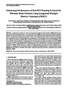
In Figure 1, the X-axis represents the OFDM transmission modes and the Y-axis shows the throughput in Mbits/s. We vary from 1 to 12 and from 1 to 3 the number of simultaneous transmissions (variable qI of the Equation (3)) in channels of 5 (dotted curves) and 20MHz (full curves in bold), respectively. It can be observed that with qI equal to 4 and 5MHz channels, i.e. a total of 20MHz occupied frequency bandwidth, a greater

TABLE III F RAME TRANSMISSION TIMES USING m8 w$

TOverhead

5MHz 10MHz 20MHz

0.38ms 0.38ms 0.38ms

TDAT A + TACK 1.404ms 0.708ms 0.36ms

TRANSMISSION MODE

TT otal 1.784ms 1.088ms 0.74ms

Throughput (f rames/s) 560.53 919.1 1351.35

120

100

Vazão(Mbps)

80

60

5MHz/qI=12 5MHz/qI=11 5MHz/qI=10 5MHz/qI=9 5MHz/qI=8 5MHz/qI=7 5MHz/qI=6 5MHz/qI=5 5MHz/qI=4 5MHz/qI=3 5MHz/qI=2 5MHz/qI=1 20MHz/qI=3 20MHz/qI=2 20MHz/qI=1

40

20

m1

m2

m3

m4

m5

m6

m7

m8

Modo de transmissão

Fig. 1.

Routes aggregated throughput (5 and 20MHz channel widths). 120

100

Throughput (Mbps)

throughput than that achieved when using qI equal to 1 and 20MHz channel for all transmission modes is obtained. This gain in favor of channels of lower widths becomes more evident when comparing the throughput of 3 channels of 20MHz with the one of 12 channels of 5MHz, with both occupying a total of 60MHz. By other results, which are not shown in this paper, one can observe that higher throughput values are obtained through the use of 2, 4 and 6 channels of 10MHz when compared to the use of 1, 2 and 3 channels of 20MHz, i.e. using equivalent total frequency bandwidth. In Figure 2, qI is assigned the values 2, 4, 6, 8, 10 and 12 for channels of 5MHz and the values 1, 2, 3, 4, 5 and 6 for 10MHz channels. It is noticed that when using 5MHz channels and the same amount of bandwidth (e.g. 2 channels of 5MHz and 1 channel of 10MHz), we obtain higher throughput with 5MHz channels when compared to the obtained values with 10MHz channels. By these results, one can conclude that the throughput obtained by using multiple lower width channels is always higher than the one obtained with wider channels even when they sum up the same total amount of frequency band. This better performance can be explained from the data in Table III that shows the successful transmission time of one data and the subsequent ACK frame for each of the 802.11 channel widths. The columns 1, 2 and 3 represent the transmission channel width (w$ ), the time spent with the overhead of the MAC layer (CWM IN , DIF S and SIF S of Equation (1)) and, the time spent with the transmission of one data and ACK frames (TDAT A plus TACK of Equation (1)), respectively. The column 4 shows the total time spent in the transmission, which is calculated by adding up the values of the columns 2 and 3. Finally, the column 5 represents the obtained throughput in each of the channel widths, which is given by 1/TT otal . Note that the time spent with overhead (TOverhead ) is the same for all channel widths. In the case of TDAT A plus TACK transmission time, these values are almost doubled each time the channel width is divided by two, as presented earlier in this section. However, simultaneous transmissions of 4 frames in 4 parallel channels of 5MHz result in a throughput value (4 × 560.53 = 2242.12 f rames/s), which is higher than the one obtained for 20MHz width. This way, one realizes that despite of the increase in TDAT A and TACK times for the narrower channels, one saves the time spent with TOverhead of serial transmissions using wider channels. In this case, one obtains greater throughputs with parallel transmissions in lower channel widths for the same amount of total frequency bandwidth.

80

60

5MHz/qI=12 5MHz/qI=10 5MHz/qI=8 5MHz/qI=6 5MHz/qI=4 5MHz/qI=2 10MHz/qI=6 10MHz/qI=5 10MHz/qI=4 10MHz/qI=3 10MHz/qI=2 10MHz/qI=1

40

20

m1

m2

m3

m4

m5

m6

m7

m8

Transmission mode

Fig. 2.

Routes aggregated throughput (5 and 10MHz channel widths).

B. Impacts on Signal Range Channel width modification implies in variations of receiver sensitivity, and thus changes to the maximum distance the signal can spread being still intelligible by the receiver. Smin = SIN Rmin + 10 log10 (K × T0 × B) + NF

(4)

In Equation (4) [8], Smin is the minimum sensitivity in dBm, SN Rmin is the minimum signal-to-noise ratio required to decode the signal, K is the Boltzmann constant (1.38 × 10−20 J/K), T0 with value 290K is the absolute temperature, B (5,10 or 20MHz) is the communication channel width and NF (typical values of 10dB [2]) is the receiver noise figure and expresses the signal deterioration caused by receiver’s internal noise circuit. From Equation (4), we obtain that SIN Rmin is given by: SIN Rmin = Smin − 10 log10 (K × T0 × B) − NF

(5)

Referring to the data-sheet of an 802.11g wireless card of 3Com [9] manufacturer, it is found that for 54 Mbits/s rate (m8 mode), the minimum sensitivity for 20MHz width is −69 dBm. Substituting this value in Equation (5), together with B = 20MHz and NF = 10dB, we can found that it is necessary ∼ = 22dB of SIN Rmin to decode the signal. By applying this result in equation 4, it is found that for B

TABLE IV M INIMUM SENSITIVITY VALUES FOR 5, 10

AND

20MHz CHANNEL

4 · π · f · d0 d ) + 10 · n · log10 ( ) c d0

· · f · d0/c)

PT −PR −20 log10 (4 π 10 n

·

300 250 200 150

m7

m6

m5

m4

m3

m2

m1

Transmission mode

Fig. 3. Transmission range of 802.11 OFDM transmission modes for 5, 10 and 20MHz channel widths

(6)

In Equation (6), P L is the free space propagation path loss given by the transmission power (PT ) minus the power perceived in the receiver (PR ). The variable f is the signal frequency in Hz (2.4GHz is used), d0 is the reference distance (values 1 or 100m for medium distance communication systems [10], 1m is used), c is the light speed in vacuum (' 3 · 108 m/s), n is the propagation loss exponent and d is the separation distance between transmitter and receiver. By isolating variable d from Equation (6), we derive Equation (7) through which we can obtain the maximum distance between transmitter and receiver for a given transmission power and receiver sensitivity. In this equation, we used PT = 17 dBm [9], n equal to 2.5 and the variable PR received the minimum sensitivity values of Table IV in order to generate the curves of Figure 3. ·

350

m8

The minimum sensitivity values of Table IV when applied to log-distance path loss equation [10] can determine the maximum distance, in meters, between a source/destination communication pair.

d = 10

400

50

Channel Widths 20MHz 10MHz 5MHz -82 -85 -88 -81 -84 -87 -79 -82 -85 -77 -80 -83 -74 -77 -80 -70 -73 -76 –66 -69 -72 –65 -68 -71

P L = PT − PR = 20log10 (

5MHz 10MHz 20MHz

450

100

WIDTHS

Mode m1 m2 m3 m4 m5 m6 m7 m8

500

Transmission range (m)

equal to 5 and 10MHz, the minimum sensitivity values for m8 transmission mode are −75 dBm and −72 dBm, respectively. Thus, each time one divides channel width by two, one reduce 3 dB in minimum sensitivity to the same transmission mode. The previous calculations explain the values of minimum sensitivity found in [2] and shown in Table IV, which are close to the measurement results presented in [3].

(7)

These curves show the maximum signal range as function of used transmission modes, from m8 (shortest range) to m1 . It is observed that in all transmission modes, greater transmission ranges are obtained using smaller channel widths. Thus, a source router could need a smaller amount of hops to communicate with a destination router across a multihop route by using smaller channel widths. Another change related to the use of smaller channel widths is the variation in CSThreshold value. In the simulations of this paper, as in [11], it was used as values for CSThreshold -82, -85 and -88 dBm for channel widths of 20, 10 and 5MHz,

respectively. Using these values, as shown in Figure 3, signal interference distance goes from a value between 200 and 250 m for 20 MHz channel width to a value of almost 400 m for 5 MHz channel width. Thus, one can see that by using smaller channel widths, a router senses transmissions from farther routers. III. S IMULATION MODEL Based on [12] and [5], we modeled the wireless mesh network using a graph G(V, E) consisting of a set of vertices V = {vi }1×|V | and a set of links (or edges) E = {ei,j,c }|V |×|V |×|C| , which can be established in a set of channels C. In the network, there is a set of flows F = {fk }1×|F | , where each flow is originated in a source router vk and has as destination router vl . Each fk flow is associated with a route of the set Ro = {rok }1×|Ro| , where |Ro| = |F |. Concerning the communication channels, the IEEE 802.11 specification [2] allows the existence of 5, 10 and 20 MHz channel widths. Generalizing, we have assumed that the total frequency bandwidth (BT OT ) can be divided into a number of discrete orthogonal channels of width w$ ($ = 1, ..., |W |, where W is the set of available channel widths). In this case, for each of the existing channel width w$ , it is possible to divide the spectrum in BT OT /w$ non-overlapping channels $ of equal width, contained in a set C w$ = {cw d }1×|C w$ | . Thus, the total S number of channels in all available widths is |W | given by C = $=1 C w$ . It can be noted that channels of different widths w$ can overlap each other. To illustrate this model, we use a BT OT frequency band equal to 60 MHz and channel widths W = {w1 , w2 } of 10 and 20 MHz. For 20 MHz channels, one have three nonw1 w1 1 overlapping channels that form the set C w1 = {cw 1 , c2 , c3 }. When the same 60 MHz frequency band is divided into six non-overlapping 10 MHz channels, they comprise the set w2 w1 2 C w2 = {cw channel is 1 , ..., C6 }. It can be noted that c1 w2 w2 overlapped with the 10 MHz wide c1 and c2 channels. As in [5], we have used the designation logical link for each $ established between routers vi and vj in channel link ei,j,cw d $ cw . Also, we have called physical link ei,j,w$ the set of all d

logical links set up between routers vi and vj using channels of the same w$ width. In the rest of the paper, we use only link to designate a logical link. In the following, we enumerate the other used notations: •

•

•

Logical Links Matrix: E = w$ $ }|V |×|V |×|C| , {ei,j,cw f orall e ∈ {0, 1}, e,j,c d d represents the routers that are within communication (RXThreshold) and carrier sense (CSThreshold) ranges (it is considered that RXThreshold is equal to $ is equal to 1, router vi can CSThreshold). If ei,j,cw d $ transmit to router vj in channel cw d . To determine the elements of this matrix, the equation (7) is used to calculate the communication distance d. For that, the PR variable is assigned to the minimum sensitivity value of the transmission mode with greater transmission range of w$ channel width (e.g. in Table IV the lowest minimum sensitivity value for 5 MHz is -88 dBm). PT and n variables assume their associated values, e.g. 17 dBm and 3.0 respectively. If the Euclidean distance di,j (d variable in the equation) is less than or equal to the $ calculated RXThreshold/CSThreshold distance, ei,j,cw d assumes value 1. Transmission Times Matrix: TX = $ }|V |×|V |×|C| ∀ ei,j,cw$ {txi,j,cw ∈ R, represents d d the transmission time of B bytes data frame using a $ cw channel. Values of this matrix are calculated for d $ equal to 1. In every pair of routers that have ei,j,cw d this case, given the distance di,j , n and PT , we calculate the received power PR(i,j) of a link by isolating PR variable of Equation (6). Then, we choose for each channel width w$ , the transmission mode mn that has minimum sensitivity (Table IV) immediately below the received power PR(i,j) . The chosen transmission mode is the one which provides the lowest transmission time and therefore will be used for communication on link $ . After transmission mode selection, we use its ei,j,cw d NDBP S value (Table II) to calculate the transmission $ through Equation (1). time txi,j,cw d Channel Occupancy Times Matrix: $ }|V |×|V |×|C| ∀ ei,j,cw$ T O = {toi,j,cw ∈ R, d d $ represents airtime occupancy of channel cw d . This matrix starts with all its values set to zero, representing that there are no transmissions in the network. When $ = β, this means that routers vi and vj realize toi,j,cw d $ that cw channel is used for a period of time equal to d z (including ei,j,cw$ β. Each new occupied link ek,l,cw e d itself) that uses partially or totally the same frequency w$ band of the cd channel and is in the interference range $ makes toi,j,cw$ to be updated by equation of ei,j,cw d dP $ $ + z ∀ ei,k,cw$ = 1 ∨ toi,j,cw = toi,j,cw txk,l,cw e d d d w$ $ $ (ej,k,cw = 1) ∨ (e = 1) ∨ (ej,l,cw = 1). i,l,cd d d The values of this matrix are used to calculate routes throughput and choose the channels with less airtime occupancy to be used by each new admitted network link.

It is considered that all routers have information about the maximum frequency bandwidth that a physical link may occupy (BM AX ). For example, BM AX equal to 20 MHz represents that a physical link ei,j,w$ can transmit with a maximum of qI = BM AX /w$ radio interfaces. Thus, if BM AX = 20MHz and w$ is equal to 5, 10 or 20 MHz, it can be used 4, 2 or 1 radio interfaces in a physical link, respectively. To calculate the throughput obtained in different routes we use the model in [13], which is extended in this work to scenarios composed of multiple transmission channels and multiple channel widths.

Route I

link 1

link 2

w c1 1

w c2 1

t1=6s

t2=6s

link 3 1 cw 3

t3=6s

link 4 w c1 1 t4=6s

cw1 2

Route II

cw1 1 t1=6s

w c2 1 t2=6s

1 cw 3

t3=6s

w c2 2 t5=t6=10s

Fig. 4.

Thoughput calculation model

In Figure 4, it is assumed that all links are within interference range of each other. The route I is composed of 4 links that occupy the channels c1 , c2 , c3 and c1 , respectively. All links have w1 width and frame transmission time equal to 6s. In this case, the throughput is equal to the lowest capacity of the links that compose the route, which is given by 1 1 1 1 min{Ca1 , Ca2 , Ca3 , Ca4 } = min{ (t1+t4) , t2 , t3 , t1+t4 } = 1 12 , where Ca is the link capacity. Note that links 1 and 4 have the lowest capacity since they share the same channel c1 . In the route II, the link 4 is replaced by a new physical link composed of c1 and c2 channels of w2 = w1 /2 width. It 1 is important to note that the cw 1 channel occupies the same w2 w2 frequency band of c1 and c2 channels. Also, the latter two channels have higher transmission airtimes ( t5 = t6 = 10s) since they are narrower. In this case, the throughput of route II 1 1 1 2 1 is given by min{ (t1+t5) , t2 , t3 , (t1+t5) } = 16 . It is observed that the throughput calculation of link 4 has a value 2 in the numerator, since two concurrent frames are transmitted using the 2 non-overlapping channels of this new link. In the Section V, we perform calculations similar to the previous example to determine the throughput of some established routes. In this case, the Equation (8), with its respective qI (amount of physical link interfaces) and B (data frame size) values, is used to determine the capacity of each used link. In the denominator of this equation, we use the values of the T O matrix to include the occupancy time perceived by links $ that compose the physical link ei,j,w . It should be ei,j,cw $ d noted that contrasting with the examples shown in Figure 4, in these calculations the links of a route could share the same channel, and hence its occupancy time, with links of other routes, as predicted in the calculations of T O matrix.

$ Caw qI =

qI · B · 8 toi,j,cw$

(8)

this algorithm, the links’ occupation and then the throughput of each route can be calculated, as described in Section III.

d

Algorithm 1: Choice of metric and channel width of links

IV. S ELECTION OF H IGHER T HROUGHPUT ROUTES According to Section II-A, the maximum throughput of a wireless mesh node is influenced by the amount of radio interfaces and the channel width used in each interface. Thus, in order to consider these new variables in route selection we have extended the Medium Time Metric (MTM) [6], creating the Burst per MTM metric (B-MTM). In the proposed metric, each physical link (ei,j,w$ ) is associated with a weight that is inversely proportional to the throughput of the physical link, according to the Equation (9). In this equation, the variable w$ ,mn VqI , defined in Equation (3), represents the obtained throughput through the use of qI communication interfaces, where each one transmit in one channel of w$ width using the mm transmission mode. The MTM metric assigns a weight to each link that is proportional to the data frame transmission time [6]. Thus, it uses the values of the T T w$ ,mn variable from Equation (3) for this assignment. According to the values in Table III, the MTM metric chooses logical links with higher channel widths (e.g. 20MHz) since these logical links have lower transmission times. However, as shown in Section II, for a given value of frequency bandwidth, when we use channels of greater width we obtain smaller values of throughput when compared to the use of concurrent transmissions using multiple lower width channels. Therefore, we propose the B-MTM metric that favors the selection of physical links composed of multiple interfaces for burst transmission using narrower qI channels. In the Equation (9), B-M T Mi,j,w represents the $ metric value for a physical link between vi and vj routers using qI interfaces of w$ channel width. qI B-M T Mi,j,w = $

1 w$ ,mn VqI

(9)

The values of the B-MTM, MTM or MNH metrics are determined in Algorithm 14 that stores the metric values for each channel width w$ and for each physical link ei,j,w$ in the matrix called metricM atrix (line 6). After that, for each pair of nodes i, j the algorithm extracts from metricM atrix the lowest metric value (line 11) and stores the extracted metric value and corresponding channel width (lines 12 and 13, respectively). The matrix betterLinkM etricM atrix, that contains the lowest calculated metric value for each pair of nodes i, j, is applied to Dijkstra’s algorithm (line 21) to determine the hops that compose each route rk . Finally, in line 25, the algorithm extracts from the matrix betterChanW idthM atrix the values of channel width to be used in each hop of each route rk . The previously extracted values are stored in a vector chanW idthOf HopsOf Route(k). After executing 4 When using MTM or MNH metrics, the values of TX and E matrices for each physical link are used in the right side of the equation of line 6, respectively. In the case of B-MTM metric, were used the values calculated from Equation(9).

1 //Calculate metric values for all physical links and //channel widths 2 foreach Channel width w$ do 3 forall Physical link ei,j,w$ do 4 //Applied the values M T Mi,j,w$ or M N Si,j,w$ 5 // when using the MTM or MNH metrics qI metricMatrix(i,j,w$ ) = B-M T Mi,j,w ; 6 $ 7 //Calculate the smallest metric value and 8 //corresponding channel width w$ 9 forall Pair of nodes i, j do 10 //min returns the smallest metric and the corresponding w$ value 11 (betterLinkMetric, betterChanWidth) = min(metricMatrix(i, j, w$ )); 12 betterLinkMetricMatrix(i, j)=betterLinkMetric; 13 betterChanWidthMatrix(i, j)=betterChanWidth; 14 //Determines the hops for each route rok and the 15 //channel width of each hop 16 foreach Flow fk do 17 source=vk ; 18 destination=vl ; 19 //Uses Dijkstra’s algorithm to determine the hops 20 //of each route 21 hopsOfRoute(k)=dijkstra(source,destination,betterLinkMetricMatrix); 22 //Extracts from betterChanWidthMatrix the values 23 //of the channel widths of each hop of the route k 24 //and stores the result in chanWidthOfRouteHops(k) 25 chanWidthOfHopsOfRoute(k) = 26 extractsChanWidthOfHopsOfRoute(hopsOfRoute(k), betterChanWidthMatrix);

V. S IMULATIONS As evaluation scenario of the proposal, we have used an area of 1000m × 1000m where 100 routers are randomly spread. The number of flows fk is varied from 1 to 10, where each flow has source and destination routers randomly selected. The frame size is 2000 bytes and the path loss exponent (n) is equal to 2.5. BT OT and BM AX variables are assigned to 60MHz and 20MHz, respectively. Hence, three, six or twelve channels of 20, 10 and 5MHz are available for transmission, respectively. Thus, routers can use 1, 2 or 4 interfaces in each physical link. The average result of 100 simulations with a confidence interval of 95% is presented below. Figures 5 and 6 show results for routers equipped with 4 transmission interfaces, while Figures 7 and 8 exhibit results for routers equipped with 2 and 8 transmission interfaces, respectively. In Figure 5, the abscissa shows the number of flows/routes and the coordinates depicts the resulting throughput in Mbits/s. It can be seen that the B-MTM metric with 5, 10 and 20MHz channels obtains higher values of aggregate throughput for all quantities of routes (rok , k = 1, ..., 10), when compared with the MTM and MNH metrics. For evaluation purposes and how can be seen in the figures, we simulated one first situation where B-MTM metric is used only with 5MHz channels and, a second situation where MNH metric is used only with 20MHz channels. The Figure 6 shows the average number of hops obtained for each configuration described above. The X-axis represents the number of used routes and the Y-axis the average number

a fewer number of hops when compared with B-MTM metric with 5, 10 and 20MHz channels. This result comes from the greater transmission range of 5MHz channels which reduces the number of hops between source and destination.

B−MTM metric / 5,10 and 20MHz channels MTM metric / 5, 10 and 20MHz channels B−MTM metric / Only 5MHz channels MNH metric / Only 20MHz channels MNH metric / 5, 10 and 20MHz channels

50

Throughput (Mbps)

40

30 B−MTM metric / 5,10 and 20MHz channels MTM metric / 5, 10 and 20MHz channels B−MTM metric / Only 5MHz channels MNH metric / Only 20MHz channels MNH metric / 5, 10 and 20MHz channels

50 20

0 0

2

4

6 Number of routes

8

10

Throughput (Mbps)

40 10

Fig. 5. Routes’ aggregate throughput (rok from 1 to 10, BT OT = 60MHz and 4 interfaces/router).

20

10

0

8

0

MTM metric / 5, 10 and 20MHz channels MNH metric / Only 20MHz channels B−MTM metric / 5, 10 and 20MHz channels B−MTM metric / Only 5MHz channels MNH metric / 5,10 and 20MHz channels

7 6

2

4

6 Number of routes

8

10


5 4 B−MTM metric / 5,10 and 20MHz channels B−MTM metric / Only 5MHz channels MTM metric / 5, 10 and 20MHz channels MNH metric / 5, 10 and 20MHz channels MNH metric / Only 20MHz channels

50

3 2

40 1 0 0

2

4

6 Number of routes

8

10

Fig. 6. Average number of hops per route (rok from 1 to 10, BT OT = 60MHz and 4 interfaces/router).

of hops. It is observed that the MTM metric, with 5, 10 and 20MHz channels, selects routes with higher number of hops when compared to other metrics. This occurs because the MTM metric assigns lower weights to links that use channels of 20 MHz width, because these links have lower transmission times (Table III). Since 20 MHz channel width has smaller transmission ranges (Figure 3), the number of hops between source and destination becomes larger. Conversely, the MNH metric with 5, 10 and 20 MHz channels presents the lower average number of hops for all quantities of routes when compared to the other metrics. This result is explained by the fact that links of 5 MHz channel width are preferred, since these links have greater transmission range. By using the MNH metric with 20 MHz channels, one can observe a lower average number of hops when compared to the MTM metric with 5, 10 and 20 MHz channels. This is due to the MTM to give priority to links of 20MHz width while the MNH metric choose routes with fewer hops with the same channel width. The B-MTM metric obtains intermediate values in the amount of hops since routes with fewer hops or smaller capacities, such as those that use larger channel widths, are not chosen. Finally, in the case of B-MTM metric with only 5MHz channels, one can observe

Throughput (Mbps)

Average number of hops per route

30

30

20

10

0 0

2

4

6 Number of routes

8

10


In Figure 7 one can observe greater values of aggregated throughput when using B-MTM and MTM metrics, both with 5, 10 and 20MHz. This is because the fewer available number of communication interfaces (e.g. 2 interfaces). In this case, both metrics tend to choose the 20 MHz channel width aiming to take advance of the available frequency bandwidth. In the case of Figure 8, is coincident the greater value of aggregated throughput when applying the B-MTM metric with 5, 10 and 20MHz and the B-MTM metric when employing only 5MHz channels. Due to the greater number of available transmission interfaces in each router and since one can obtain a greater throughput value when using parallel transmissions in narrower channels, the B-MTM metric tends to choose 5 MHz channels. We simulated a second scenario that differs from the first in relation to the BT OT variable, that now assumes the value 80MHz. The results are showed in figures 9 and 10 for routers

R EFERENCES

B−MTM metric / 5,10 and 20MHz channels MTM metric / 5, 10 and 20MHz channels B−MTM metric / Only 5MHz channels MNH metric / Only 20MHz channels MNH metric / 5, 10 and 20MHz channels

50

Vazão (Mbps)

40

30

20

10

0 0

2

4 6 Quantidade de Rotas

8

10


60 B−MTM metric / 5,10 and 20MHz channels B−MTM metric / Only 5MHz channels MTM metric / 5, 10 and 20MHz channels MNH metric / 5, 10 and 20MHz channels MNH metric / Only 20MHz channels

Throughput (Mbps)

50

40

30

20

10

0 0

2

4

6 Numer of routes

8

10


equipped with 4 and 8 transmission interfaces, respectively. It is observed that the B-MTM metric makes better use of a larger frequency bandwidth, thus obtaining a greater amount of aggregate throughput for all number of routes, when compared with the other metrics. VI. C ONCLUSION This paper studies the impact of changing channel width in 802.11 networks with OFDM physical layer. From the observations, a model to simulate networks with these features was established. Following, a routing metric (B-MTM) for choosing routes of higher throughput and an algorithm for channel width selection were proposed. Simulations to compare the obtained throughput by the B-MTM, MNH (Minimum Number of Hops) and MTM (Medium Time Metric) metrics were performed. The results show the effectiveness of the proposal in determining routes of higher throughput. Future studies aim to treat the choice of routes in multiple channel widths networks as an optimization problem.

[1] H. Arslan and J. Mitola, III, “Special issue: Cognitive radio, softwaredefined radio, and adaptive wireless systems: Guest editorials,” Wirel. Commun. Mob. Comput., vol. 7, no. 9, pp. 1033–1035, 2007. [2] “Wireless LAN Medium Access Control (MAC) and Physical Layer (PHY) Specifications,” IEEE Standard 802.11, 2007. [3] R. Chandra, R. Mahajan, T. Moscibroda, R. Raghavendra, and P. Bahl, “A case for adapting channel width in wireless networks,” in SIGCOMM Comput. Commun. Rev., vol. 38, no. 4. New York, NY, USA: ACM, 2008, pp. 135–146. [4] Y. Yuan, P. Bahl, R. Chandra, P. A. Chou, J. I. Ferrell, T. Moscibroda, S. Narlanka, and Y. Wu, “Knows: Kognitiv networking over white spaces,” in Proceedings of IEEE DySPAN 2007, Apr. 2007. [5] L. Li and C. Zhang, “Optimal channel width adaptation, logical topology design, and routing in wireless mesh networks,” EURASIP - Journal on Wireless Communications and Networking, vol. 2009, 2009. [6] B. Awerbuch, D. Holmer, and H. Rubens, “The medium time metric: High throughput route selection in multi-rate ad hoc wireless networks,” Mobile Networks and Applications (MONET) Journal, Special Issue on Internet Wireless Access: 802.11 and Beyond, vol. 2004, pp. 253–266, 2004. [7] R. Prasad, OFDM for Wireless Communications Systems. Boston: Artech House, 2004. [8] Q. Gu, RF Systems Design of Transceivers for Wireless Communications. New York: Springer, 2005. [9] 3Com, “3com 11a/b/g wireless pc card datasheet,” http://www.3com. com/other/pdfs/products/en\ US/400813.pdf, apr 2004. [10] T. Rappaport, Wireless Communications: Principles and Practice. Upper Saddle River, NJ, USA: Prentice Hall PTR, 2001. [11] P. Piggin, “Ieee p802.19 wireless coexistence - parameters for simulation of wireless coexistence in the us 3.65ghz band.” http://ieee802.org/ 19/pub/2007/19-07-0011-10-0000-Parameters-for-Simulation.doc, jul 2007. [12] F. Ye, Q. Chen, and Z. Niu, “End-to-end throughput-aware channel assignment in multi-radio wireless mesh networks,” in Global Telecommunications Conference, 2007. GLOBECOM ’07. IEEE, Nov. 2007, pp. 1375–1379. [13] T. Salonidis, M. Garetto, A. Saha, and E. Knightly, “Identifying high throughput paths in 802.11 mesh networks: a model-based approach,” in Network Protocols, 2007. ICNP 2007. IEEE International Conference on, Oct 2007, pp. 21–30.