1
Routing Protocols for Self-Organizing Hierarchical Ad-Hoc Wireless Networks S. Zhao, K. Tepe, I. Seskar and D. Raychaudhuri WINLAB, Rutgers University 73 Brett Road, Piscataway, NJ 08854
[email protected] Abstract— A novel self-organizing hierarchical architecture is proposed for improving the scalability properties of adhoc wireless networks. This paper focuses on the design and evaluation of routing protocols applicable to this class of hierarchical ad-hoc networks. The performance of a hierarchical network with the popular dynamic source routing (DSR) protocol is evaluated and compared with that of a conventional “flat” ad-hoc networks using an ns-2 simulation model. The results for an example sensor network scenario show significant capacity increases with the hierarchical architecture (∼4:1). Alternative routing metrics that account for energy efficiency are also considered briefly, and the effect on user performance and system capacity are given for a specific example.
I. Introduction Ad-hoc networks in which radio nodes communicate via multi-hop routing have long been considered for tactical military communications without wired infrastructure. More recently, ad-hoc radio techniques have migrated to dual-use and commercial scenarios such as sensor networks, home computing and public wireless LAN. While ad-hoc wireless networks offer important rapid deployment and cost benefits, the traditional “flat” multi-hop routing approach does not scale well, i.e. throughput per node decreases and delay increases as the number of nodes in the system becomes large. In [1], Gupta and Kumar obtain an upper bound on the throughput √ of ad-hoc wireless networks, which decreases as O(1/ n) per node, as the number of nodes (n) increases. This motivates consideration of more scalable ad-hoc network architecures, possibly based on hierarchical approaches. In addition, potential ad-hoc network applications (such as sensor arrays) involve traffic flows to and from the Internet in addition to peer-to-peer communication between nodes, thus requiring effective hierarchical integration with the wired infrastructure. Based on the above considerations, we are investigating a new class of self-organizing hierarchical ad-hoc wireless networks with improved scaling properties and more natural integration with the wired Internet. The network is designed to provide hierarchical scaling of throughput with bounded delay, while retaining some of the flexibility and cost advantages of an infrastructure-less ad-hoc network. Major design considerations for the proposed hierarchical ad-hoc network include a discovery and topology establishment protocol for self-organization, a MAC protocol for efficient use of radio resources, and a routing protocol to support multi-hop packet transport. Many routing protocols have been proposed for ad-hoc networks: DSR [2], AODV (Ad-hoc On-demand Distance Vector) [3], TORA (Temporally Ordered Routing Algorithm) [4] etc. Most of them are designed for the “flat” Research supported in part by NJ Commission of Science and Technology Grant #03-2042-007-12. K. Tepe is now with ECE Dept., Univ. of Windsor, Windsor, CA.
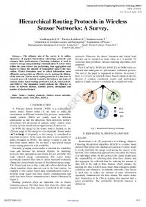
architecure, although they may also be used in hierarchical scenarios with appropriate modification. Some routing protocols have also been developed especially for hierarchical architecture, such as ARC (Adaptive Routing using Clusters) protocol [5]. Our goal is to evaluate how different routing protocols work in the hierarchical mode, and what the resulting system capacity and user performance would be. One aspect is to evaluate the relative applicability of popular ad-hoc routing protocols such as DSR to the hierarchical network under consideration. A second issue is that of selecting appropriate routing metrics that reflect additional performance criteria such as energy efficiency [7]. This paper reports on early results with an ns-2 simulation model used to compare hierarchical and flat ad-hoc networks with DSR routing. Alternative routing metrics for energy efficiency are also considered briefly, and example performance results are provided. The rest of this paper is organized as follows. In the next section we introduce the proposed hierarchical ad-hoc network. In section 3 we discuss the routing protocol and alternative energy-aware metrics. The simulation model and performance results for an example “sensor network” scenario are presented in section 4. Finally, section 5 summarizes the main results and outlines our future work. II. Hierarchical Ad-hoc Network The proposed network architecture is based on three tiers of wireless devices: low-power “sensor nodes” with limited functionality, higher-power “radio forwarding nodes” that route packets between radio links, and “access points” that route packets between radio links and the wired infrastructure. Their functions are summarized below (see Fig. 1).
Fig. 1. Hierarchical ad-hoc network architecture
Sensor Node (SN): The sensor node is in the lowest tier and (unlike the traditional flat network model) does not offer multi-hop routing capability to its neighbors. SN’s route packets via higher tier nodes, which may be either forwarding nodes or access points. •
2
• Forwarding Node (FN): The forwarding node is the second tier that offers multi-hop routing capability to nearby SN’s or other FN’s. The FN has two wireless interfaces, one communicates with lower tier nodes (SN’s) and the other connects to higher tier nodes (FN’s and AP’s). • Access Point (AP): The access point is the highest tier in the network, and has both wireless and wired interfaces (similar to those used in conventional 802.11b wireless LAN’s). AP’s provide multi-hop routing for packets from SN’s and FN’s within radio range, in addition to routing data to and from the wired Internet.
III. Routing Protocol and Metrics From the routing point of view, hierarchy can significantly increase the routing efficiency by reducing the number of nodes involving in the routing and the number of control packets generated by routing protocols. Thus the network throughput can be increased (for given radio link capabilities), data packet delay can be improved, and routing overhead can be reduced. We divide the hierarchical ad-hoc networking functionality into three components: MAC, discovery1 and routing. In this paper, we focus on routing with the assumption that the other two functions work according to their nominal designs. In particular, all nodes in the system operate with the standard 802.11b ad-hoc mode MAC with specified power and range. The discovery protocol used in the system is assumed to provide an idealized hierarchical network topology, and then maintain and optimize the topology, which may change due to the node movements and varying network traffic. After studying and comparing different ad-hoc routing protocols and the specific requirements of the proposed hierarchical network, we have some considerations for the routing protocol. Firstly, routing updates should be “ondemand” to minimize routing overhead. The DSR method used in many ad-hoc networks is thus a candidate, although source routing may increase the number of routing overhead bytes in large sensor networks with moderate node mobility. Alternative on-demand routing protocols such as AODV, as well as protocols explicitly designed for hierarchical networks (e.g. ARC) also need to be evaluated and compared with DSR for the scenario under consideration. When calculating the routing cost, the energy consumption of nodes, the number of hops reaching the destination, the available radio bandwidth, the link latency and the network traffic load, can be used as parameters. It may also be possible to devise integrated MAC/routing policies with metrics related to dynamically observed radio link parameters. We start with DSR and identify protocol and algorithmic extensions necessary for efficient operation in the hierarchical environment. Hierarchical ad-hoc network system capacity and performance are evaluated for an example “sensor network” scenario using the ns-2 network simulator. The results obtained are compared with those of a conventional “flat” ad-hoc network in order to estimate the potential increase in system capacity with the three-tier hierarchy. 1 Preliminary information about this discovery protocol can be found in D. Raychaudhuri, “4G Network Architecture: 3G/WLAN Interworking, Infostations and Beyond”, PIMRC’02 Plenary Speech, Lisbon, Sept 2002. The presentation can be downloaded at: www.winlab.rutgers.edu.
IV. Methodology and Simulation Model Our experiments were conducted using the Monarch extensions to the ns-2 network simulator. We use an identical spatial node distribution, traffic flow matrix and mobility scenarios for the hierarchical and flat networks. A. Hierarchical Ad-hoc Network and DSR Modification The ns-2 simulator only supports conventional flat adhoc networks, which means that all mobile nodes have the same functionalities, including the routing capability. In order to implement our hierarchical network in ns-2 and run DSR on it, we make the following modifications: 1) In the proposed hierarchical ad-hoc network, an idealized discovery protocol is used to establish and maintain the hierarchical topology. When performing experiments on routing, we make the following assumptions in order to evaluate the system performance as a whole: a. In the hierarchical ad-hoc network, nodes are assumed to organize themselves into clusters. For simplicity in this study, we assume that there is only one “gateway AP” per cluster associated with an arbitrary number of FN’s and SN’s. When a SN wishes to communicate with any other node outside its cluster, packets must go through the gateway AP. We assume that any FN or SN can only belong to one cluster, i.e., it only has one unique gateway AP. If an FN or SN is within the radio transmission range of its gateway AP, it is connected to the gateway AP directly; otherwise, the connection is through one or more intermediate FN’s. If there is more than one AP within the radio transmission range of an FN or SN, the FN or SN are assumed to connect only through the gateway AP. This assumes that the discovery protocol supports identification of gateway AP’s and association of related FN’s and SN’s in each cluster. b. We assume that we have an optimized self-organizing hierarchical topology during the routing simulations. In particular, we assume that the clusters are created and maintained with balanced traffic load. Meanwhile, any FN or SN can move out of its original cluster and join a new cluster due to its movement; the discovery protocol will also take care of this topology change. Under these assumptions, we can simply implement the hierarchical adhoc network by dividing the simulated site into a certain number of clusters, with the gateway AP in the center of each cluster. Our simulation scenarios are run with approximately the same number of nodes in each cluster and the same traffic pattern in the nodes. 2) The SN is modeled as a simple mobile node without multi-hop routing capability offered to neighbors. During DSR route discovery procedure, SN’s ignore route request messages they may receive. And when a node operating in promiscuous mode overhears a route, before it adds this route to its cache, it makes sure that there is no SN contained in the route. These modifications assure that any SN will not be used as an intermediate node to forward packets for other nodes. 3) The FN has full multi-hop routing capability. Note that in the present simulation model, each FN only forwards packets to other nodes within the same cluster. 4) Wired AP links are assumed to be high-speed links (such as ∼100 Mbps supported by an upstream Ethernet switch). Wired network congestion is ignored in our model, and the packet error rate is set to zero for wired connec-
3
tions. Delays caused by a wired link between AP’s are obtained by dividing the packet size by the link speed. As explained ealier, the gateway AP receives all packets sent by the nodes in its cluster, no matter which AP is the eventual destination (this is because packets can be forwarded between AP’s over high bandwidth wired links with minimal routing cost). For packets not directed to the gateway AP, end-to-end delay is calculated as the sum of the delays in the wireless network and in the wired network. B. Hierarchical Sensor Network Simulation Model The simulation study considers an example sensor network deployed over a square geographical coverage area with dimension 1000m × 1000m. We divide the coverage area into four 500m × 500m smaller squares, each corresponding to a cluster with one gateway AP and several FN’s and SN’s. The gateway AP is static and located in the center of each small square. Thus, there are 4 AP’s in the simulated area of coverage. The FN’s and SN’s are randomly placed within the clusters. In this model, we assume a uniform density of SN’s and FN’s, with a nominal value of 20 FN’s and 100 SN’s spread over the entire coverage area. The FN’s move according to the random waypoint model [2] with a randomly chosen speed (uniformly distributed between 0-1 m/s) and pause time 0 (which means that FN’s do not stop during their journey). Half of the SN’s are static. The remaining half of the SN’s move according to the same random waypoint model as the FN’s. These parameters have been chosen to an example sensor network scenario, but are by no means unique. Other sensor network scenarios and traffic models will be considered in the future work. C. Traffic Pattern Sensor nodes generate traffic according to an exponential on/off model [6]. Packets are sent at a specific rate during “on” periods, and no packet is sent during “off” periods. Both “on” and “off” periods are taken from an exponential distribution. We choose the average “on” time (burst time) to be 500 ms, the average “off” time (idle time) to be 500 ms, and the packet size to be 64 bytes per packet. The number of packets per second generated by SN’s is varied as an input parameter in order to gradually increase the offered load to the network as a whole. All traffic in the sensor network scenario is originated at SN’s, and 80% of this traffic is assumed to be bound for a server within the Internet, accessed through a gateway AP; the remaining 20% of SN traffic is assumed to be routed to other SN’s in the network, accessed via one or more FN’s and AP’s. Each SN can simultaneous support up to two traffic flows to different destinations. Traffic in the network is assumed to be uniform and balanced. D. Energy Cost Metrics Standard DSR as implemented in ns-2 uses the number of hops as metric to make routing decisions. This metric tends to choose the route with the minimum data packet delay. In addition to delay, we may have to consider other system performance such as throughput and energy consumption. Since energy is a serious constraint in sensor networks, it may be appropriate to use energy cost as an alternative link metric. When such a metric is used, the sytem will tend to favor routes with multiple SN-FN-FNAP hops rather than a direct high-power link from SN to
AP. Note that use of energy-aware routing metrics implies the existence of reasonably effective power control at the 802.11b link/physical level. Such power control may also be expected to improve MAC layer efficiency in the network. V. Performance Results A. Performance Metrics In order to compare the system performance of hierarchical and flat ad-hoc networks, we focus on the following four performance metrics: • Packet delivery fraction: measured as a ratio of the number of data packets delivered to their eventual destinations and the number of data packets generated by sources. • Average end-to-end delay: includes all possible delays caused by buffering during route discovery, queuing at the interface queue, retransmission delays at MAC, propagation delay and transfer times. If the data packets go through a wired link, the delay caused by the wired link is also taken into account. • Normalized routing load: measured as the number of routing packets transmitted per data packet delivered at destinations. Each hop is counted as one transmission for both routing and data packets sent over multiple hops. • System throughput: measured as the total number of useful data (in bps) received at traffic destinations, averaged over the duration of the entire simulation. B. Results and Discussions A series of simulation experiments for the sensor network scenario were conducted using the system model and parameters outlined above. The key parameters are summarized in Table I below. TABLE I Simulation parameters Coverage area # of clusters; SN’s; FN’s; AP’s Radio PHY ; Radio range MAC AP-AP link speed # of communication pairs # of pkts/s generated Packet size % of SN-Internet traffic
1000m × 1000m 4; 100; 20; 4 1 Mbps; 250 m ad-hoc 802.11b 100 Mbps 40 1,4,8,12,16,24,32 64 bytes 100%
From Fig. 2 (a) which shows throughput as a function of offered load from the sensors (for 40 SN-AP communicating pairs2 ), we see that the hierarchical system begins to saturate when the packet generation rate reaches 16 pkts/s; while the flat system saturates at about 4 pkts/s. For the 802.11b bandwidth of 1 Mbps used in the study, system capacities are found to be ∼ 320 kbps for the hierarchical case and ∼ 77 kbps for the flat case, respectively. It is observed that the system capacity increases by a factor of ∼ 4× if the proposed hierarchical architecture is adopted. Clearly, this is a significant scaling increase over the relatively low 77 kbps obtained with flat ad-hoc network. The exact factor by which the capacity increases will depend upon several factors including topology, spatial distribution of SN’s, the ratio of SN’s to FN’s and AP’s, etc. The gain is expected to be in the range of ∼ 3 − 5× 2 The simulations were repeated for two other cases corresponding to 20 and 60 communication pairs and results similar to the 40-pair case were observed.
4
for various typical sensor network scenarios that we have been considering. Corresponding average end-to-end delay and packet delivery fraction curves are shown in Fig. 2 (b) and (c), while Fig. 3 shows delay-throughput curves which summarize system capacity and performance as a whole. The figures show that the hierarchical network has better performance in terms of the performance metrics that we evaluate when compared with the flat ad-hoc network. Each SN communicates through a few FN’s and a single gateway AP, thus reducing the number of hops to reach the Internet, where most packets from sensors have their destinations (100% in this study). In addition, SN’s do not join the protocol for distribution of routing messages, thus reducing routing overhead significantly. Of course, the capacity increase comes at the expense of increased hardware (FN’s and AP’s) relative to a flat sensor network, and in that sense it is not an “apples-to-apples” comparison. A pragmatic analysis of the results indicates that there is a need for some support infrastructure components (i.e. FN’s and AP’s) for better sensor network performance and increased system capacity. If the hierarchical ad-hoc network is implemented properly, it retains many of the self-organization and robustness advantages of pure ad-hoc routing among sensors while providing major gains in achievable throughput and performance. 5
x 10
4 Avg delay (simulated s)
3.5 Throughput (bps)
3 2.5 2 1.5 1 Hier Flat
0.5 0 0
Hier Flat
3 2 1 0 0
10 20 30 Packet rate (pkts/s)
10 20 30 Packet rate (pkts/s) (b)
0.25
0.8
0.2
Routing overhead
Pkt delivery fraction
(a)
1
0.6 0.4 0.2 0 0
Hier Flat
10 20 30 Packet rate (pkts/s)
Hier Flat
0.15 0.1 0.05 0 0
10 20 30 Packet rate (pkts/s)
(c)
(d)
Fig. 2. Simulation results for 40 communication pairs
the actual power required to transmit on each radio link. In particular, the energy cost is a function of the sum of the transmission power required to reach the next hop through the path. From the results for 12 pkts/s shown in Table II, it is observed that the network with energy-aware routing metric helps reduce power consumption (the average energy cost per data packet is about 15-20% less) at the nodes at the expense of somewhat lower throughput and higher delay. This result matches our expectations, and leads us to expect that combined link metrics with a mix of both hop-count and energy can be used to further tune the performance vs. energy consumption at sensor nodes. TABLE II Simulation results of hop-count and energy-cost metircs Metric Delivery fraction Throughput (bps) Average delay (s)
Avg end−to−end delay (s)
3.5
We have compared the performance of DSR routing methods for the traditional flat and the proposed hierarchical ad-hoc networks. We observed that the self-organizing hierarchical ad-hoc network performs well with suitably modified DSR protocol, and generally results in significant improvements in both system capacity and end-user performance measures (such as delay and packet delivery fraction). Of course, the hierarchical architecture does require additional investment in forwarding node and access point equipment. The simulations using energy cost metric show that the power consumption at sensor nodes can be traded off against throughput and delay. It is remarked that we have presented preliminary results here from work in progress, and expect to address several open architectural and design optimization issues in future work. These topics include evaluation of alternative classes of ad-hoc routing (such as AODV) in the hierarchical scenario, design of more customized hierarchical routing protocols, more integrated consideration of MAC, discovery and routing protocols, and more complete system studies of realistic sensor network scenarios. We also plan to implement selected hierarchical ad-hoc network protocols on the WINLAB sensor network testbed for the purposes of protocol validation and integration with real-world sensor applications. References [1]
3
[2]
2.5 2
[3]
1.5 1
[4]
0.5 0 0
0.5
1 1.5 2 2.5 System throughput (bps)
3
3.5 5 x 10
Fig. 3. Delay vs. throughput for 40 communication pairs
We also briefly studied the feasibility of using alternative routing metrics (such as the energy cost) within the DSR framework. Specifically, we simulated for the same model and parameters as described above, with the hop-count metric in DSR replaced by an energy metric computed from
Energy-cost 0.946 212631 0.0454
VI. Conclusions and Future Work
4 Hier flat
Hop-count 0.982 220084 0.0258
[5] [6]
[7]
P. Gupta and P. R. Kumar, “The capacity of wireless networks”, IEEE Trans. on Information Theory, Vol. 46, pp. 388404, March 2000. D. B. Johnson and D. A. Maltz, “Dynamic source routing in ad hoc wireless networks”, Mobile Computing, T. Imielinski and H. Korth, Eds. Norwell, MA: Kluwer, ch. 5, pp. 153-181, 1996. C. Perkins and E. Royer, “Ad hoc on-demand distance vector routing”, Ad hoc Networking, Addison-Wesley Publishers, Editor C. Perkins, 2000. V. D. Park and M. S. Corson, “A highly adaptive distributed routing algorithm for mobile wireless networks”, IEEE Proceedings of INFOCOM’97, April 1997. E.M. Belding-Royer, “Hierarchical Routing in Ad hoc Mobile Networks”, Wireless Communication and Mobile Computing, pp. 515-532, 2002. K. Fall and K. Varadhan, Eds., “The ns Manual”(2002). The VINT Project, UC Berkeley, LBL, USC/ISI, and Xerox PARC. [Online]. Available WWW: http://www.isi.edu/nsnam/ns/doc/ns doc.pdf S. Singh, M. Woo, and C.S. Raghavendra, “Power-aware routing in mobile ad hoc networks”, Procc. ACM MOBICOM, 1998.